Table of Contents

Buffer Analysis in GIS: Step-by-Step Proximity Mapping

Buffer analysis in GIS is one of the most useful proximity-analysis techniques for university GIS assignments. It allows you to create zones at specified distances around points, lines, or polygons and then investigate which features fall inside those zones.

For example, you might need to create a 500-meter environmental protection zone around rivers, identify schools within 1 kilometer of major roads, or determine which buildings are exposed to a flood-risk corridor.

The difficult part is often not clicking the Buffer tool. Students commonly encounter problems involving CRS and distance units, dissolve settings, buffer geometry, multiple distance zones, and Euclidean versus geodesic calculations.

This guide explains the complete workflow in QGIS and ArcGIS Pro, including the parameters you need to understand for a GIS lab assignment.

What You Will Learn

What buffer analysis is and why it is useful
Euclidean vs geodesic buffering
Fixed-distance vs variable-distance buffers
Single-ring vs multi-ring buffers
How to create buffers in QGIS
How to create buffers in ArcGIS Pro
How dissolve, end-cap, and join settings affect results
How to avoid CRS-related distance errors
How to use buffers in a practical environmental analysis

What Is Buffer Analysis in GIS?

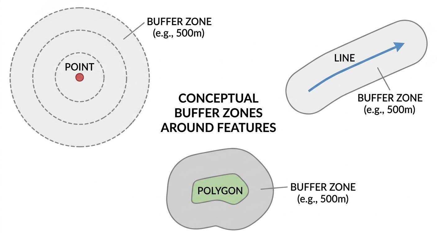
A buffer is a zone created around a geographic feature at a specified distance.

The input feature can be:

Point — such as a school, hospital, well, or weather station
Line — such as a river, road, pipeline, or railway
Polygon — such as a protected area, lake, or urban boundary

For example, a 500-meter buffer around a river creates a zone extending 500 meters outward from the river’s geometry.

Buffer analysis is useful because it converts a simple distance requirement into a spatial dataset that can be queried, measured, intersected, or overlaid with other GIS layers.

Common Applications

Students encounter buffer analysis in many disciplines.

Environmental science:

Protection zones around rivers
Wildlife corridor analysis
Pollution impact zones
Wetland protection

Urban planning:

Schools within walking-distance zones
Development restrictions around infrastructure
Public-service accessibility

Transportation:

Properties near roads
Railway impact zones
Road safety analysis

Disaster management:

Areas near flood channels
Hazard zones around volcanoes
Evacuation planning

Public health:

Population within a specified distance of healthcare facilities
Exposure zones around pollution sources

Buffer Analysis in GIS: Understanding the Main Types

Before running a Buffer tool, understand what type of buffer your assignment requires.

Euclidean Buffers

A Euclidean buffer uses straight-line distance.

If you create a 500-meter buffer around a point, every location within 500 meters in the coordinate system’s distance units is included.

This is the traditional approach used for many GIS proximity analyses.

Euclidean buffers are appropriate when straight-line distance is a reasonable representation of proximity.

Geodesic Buffers

A geodesic buffer accounts for distances measured across the Earth’s curved surface.

This becomes particularly important when:

working across large geographic areas
using geographic coordinate systems
analyzing long distances
working with global datasets

For small local study areas using an appropriate projected coordinate system, a planar/Euclidean buffer may be sufficient.

Pro Tip: Don’t choose geodesic simply because it sounds more accurate. Choose the distance model that matches your geographic scale, coordinate system, and research question.

Fixed-Distance vs Variable-Distance Buffers

Fixed-Distance Buffer

A fixed-distance buffer uses the same distance for every input feature.

For example:

Create a 500-meter buffer around every river segment.

Every feature receives a 500-meter buffer.

Variable-Distance Buffer

A variable buffer uses a distance stored in an attribute field.

For example:

Road	Speed Limit	Buffer
Road A	30 km/h	20 m
Road B	60 km/h	40 m
Road C	100 km/h	100 m

The GIS software reads the distance from the relevant field.

This is useful when different features require different protection or influence distances.

Single-Ring vs Multi-Ring Buffers

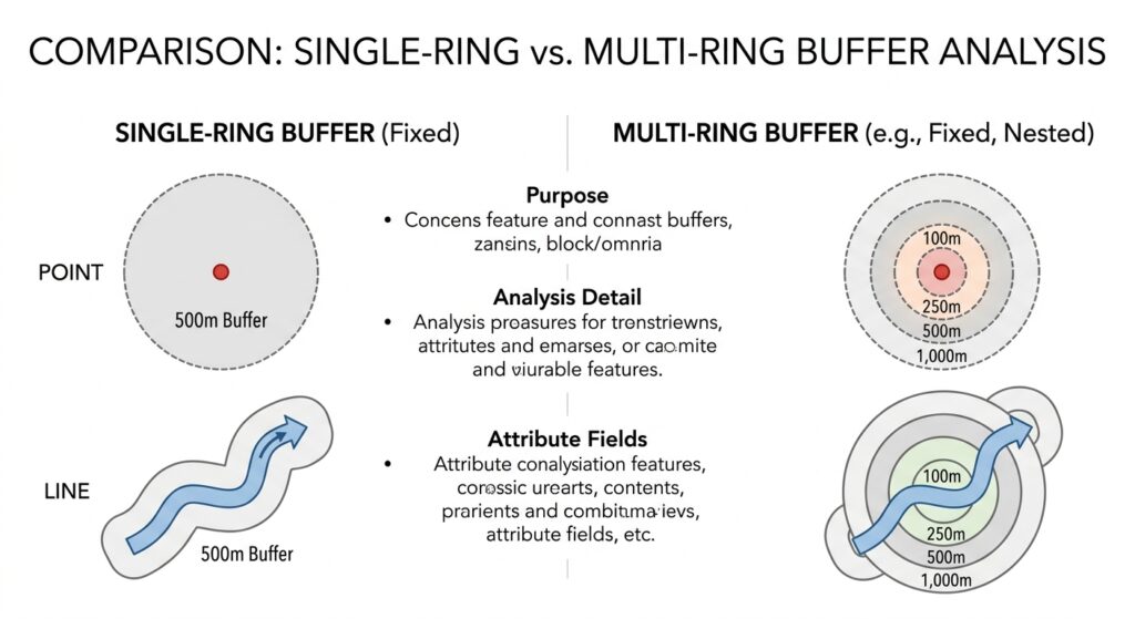
Single-Ring Buffer

A single-ring buffer creates one zone around the input.

For example:

River → 500 m buffer

Everything within that distance belongs to one buffer zone.

Multi-Ring Buffer

A multiple-ring buffer creates several distance zones.

For example:

100 m
250 m
500 m
1,000 m

This allows you to investigate how spatial relationships change with increasing distance.

]

Before Buffering: Check Your CRS

This is one of the most important steps in buffer analysis in GIS.

Suppose your layer uses a geographic coordinate system such as latitude and longitude.

The coordinates may look like:

36.8219, -1.2921

These are angular coordinates, not meters.

If your assignment says:

Create a 500-meter buffer.

you need to make sure the software is working with an appropriate distance measurement.

Use a Projected Coordinate System

For many local and regional analyses, project your data into an appropriate Projected Coordinate System (PCS) using linear units such as:

meters
feet

This makes distance-based operations easier to interpret.

[Internal Link Context: Suggest linking to related article on Geographic vs Projected CRS]

Pro Tip: A common student mistake is creating a “500-meter” buffer while the layer’s coordinate units are degrees. Always inspect the layer’s CRS and units before running the tool.

How to Perform Buffer Analysis in QGIS

QGIS provides buffer functionality through its Processing Toolbox and vector geometry tools.

Step 1: Load Your Input Layer

Open QGIS and add your point, line, or polygon layer.

For example, suppose your assignment involves rivers.

Your input layer might be:

river_streams.gpkg

Open the layer properties and verify its CRS.

Step 2: Reproject if Necessary

If your data uses geographic coordinates, create a projected version appropriate for your study area.

You can use:

Processing → Toolbox → Reproject Layer

Choose an appropriate projected CRS with meter-based units.

Save the reprojected layer as a new dataset.

Step 3: Open the Buffer Tool

Open:

Processing → Toolbox

Search for:

Buffer

Depending on your QGIS version and installed Processing providers, you may find the native vector geometry Buffer tool.

Step 4: Select the Input Layer

Choose your river layer.

Set the Distance parameter to:

500 meters

if your projected layer uses meters.

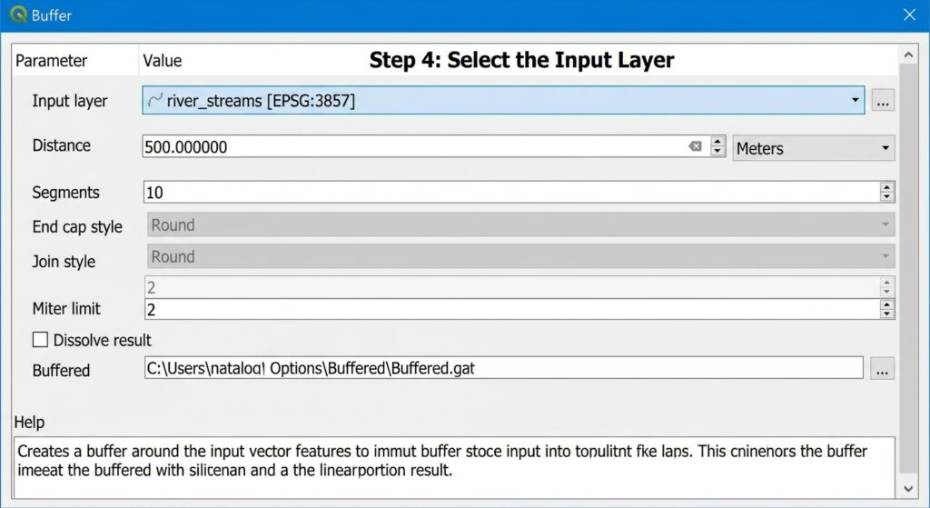
Step 5: Set the Number of Segments

For point and curved geometries, GIS software approximates curves using line segments.

A higher number of segments produces a smoother-looking buffer.

However, increasing the number unnecessarily can make the output larger and slower to process.

For a university lab, use a reasonable value and document it if required.

Understanding QGIS Buffer Settings

End Cap Style

End-cap style controls how the ends of buffered line features are constructed.

Common options include:

Round: creates rounded ends.

Flat: terminates the buffer at the end of the line.

Square: extends the buffer beyond the endpoint.

For a river or road network, the choice can influence the appearance of the resulting zone.

Join Style

Join style controls how corners are handled around line or polygon geometries.

Common options include:

Round
Miter
Bevel

Round generally produces smoother corners.

Dissolve

Dissolve controls whether overlapping buffer areas remain separate or are merged.

No Dissolve: each input feature retains its own buffer.

Dissolve All: overlapping buffers are merged into a single combined zone.

This distinction is important for analysis.

Suppose two nearby rivers each have a 500-meter buffer.

Without dissolve, you may have two overlapping polygons.

With dissolve, overlapping portions can become part of a unified protection zone.

Step 6: Run and Inspect the Buffer

Click Run.

QGIS creates a new polygon layer representing the buffer.

Inspect:

Distance
Geometry
CRS
Attribute table
Overlapping zones
Output extent

Don’t immediately assume the result is correct.

Use the measurement tools to check whether the buffer is approximately the requested distance.

How to Perform Buffer Analysis in ArcGIS Pro

ArcGIS Pro provides buffer functionality through the Analysis Tools → Proximity toolset.

Step 1: Add Your Data

Add your point, line, or polygon dataset to the ArcGIS Pro map.

Check its coordinate system before creating the buffer.

Step 2: Reproject the Data

If necessary, use:

Data → Export Features

or the Project geoprocessing tool to create a version using an appropriate projected coordinate system.

Choose a CRS with appropriate linear units for your study area.

Step 3: Open the Buffer Tool

Go to:

Analysis → Tools

Search for:

Buffer

Open the appropriate proximity tool.

Step 4: Select the Input Features

Choose your input layer.

For example:

River_Streams

Set the output feature class.

Step 5: Enter the Buffer Distance

Enter:

500 Meters

if your assignment requires a 500-meter protection zone.

ArcGIS Pro allows you to specify distance units directly, but you should still understand the coordinate system and distance model being used.

ArcGIS Pro Buffer Parameters

Dissolve Type

ArcGIS Pro provides options controlling how buffers are merged.

None: each input feature retains its own buffer.

All: overlapping buffers are dissolved into a single output feature or set of features according to the tool’s output behavior.

List: features can be dissolved based on one or more attribute fields.

Use None when you need to preserve individual relationships between buffers and input features.

Use All when your assignment requires one continuous protection or influence zone.

Method: Planar vs Geodesic

Depending on the ArcGIS Pro Buffer tool and workflow, you may encounter a choice between planar and geodesic methods.

Planar uses planar calculations based on the projected coordinate system.

Geodesic calculates distance on the Earth’s curved surface.

For large-area analyses or situations where projection distortion matters, geodesic calculations can be advantageous.

End Cap Style

For line buffers, you may encounter options such as:

Round
Flat
Square

The choice determines how the buffer terminates at line endpoints.

Side Type

Some workflows allow you to specify whether the buffer is created:

On both sides
Left side
Right side

This can be useful for transportation or linear infrastructure analysis.

Practical Student Scenario: 500-Meter River Protection Zone

Imagine your GIS assignment says:

“Create a 500-meter environmental protection zone around all major rivers and determine which settlements fall within the protected area.”

Here’s how you could approach it.

Step 1: Prepare the River Layer

Load your river/stream line layer.

Check its CRS and reproject it to an appropriate projected coordinate system using meters.

Step 2: Create the Buffer

Run the Buffer tool with:

Distance: 500 m

End Cap: Round

Join Style: Round

Dissolve: All

The result is a continuous protection-zone layer where buffers overlap.

Step 3: Add Settlement Data

Load your settlement or building-point layer.

Step 4: Select Features Within the Buffer

Use a spatial selection such as:

Select by Location

Choose settlements that intersect the 500-meter buffer.

Step 5: Calculate the Number of Exposed Settlements

Count the selected features.

You can then report something such as:

“A total of 143 mapped settlements intersect the 500-meter river protection zone.”

The exact result depends on your dataset.

Step 6: Produce the Final Map

Your map should clearly distinguish:

Rivers
Buffer zone
Settlements
Study-area boundary

Include a legend, scale bar, north arrow where appropriate, title, and data sources.

Buffer Analysis in GIS: Common Mistakes

Mistake 1: Buffering Data in Degrees

This is one of the most serious beginner mistakes.

If your layer uses longitude and latitude, blindly entering “500” does not necessarily mean 500 meters.

Check the CRS first.

Mistake 2: Using the Wrong Distance Units

A buffer of:

500 feet

is not the same as:

500 meters

Always check the units displayed by the software.

Mistake 3: Dissolving When You Shouldn’t

Dissolving removes internal boundaries between overlapping buffers.

That can be useful for creating a single protection zone but problematic if your assignment requires individual buffers for each feature.

Mistake 4: Ignoring Projection Distortion

Even when your software produces a technically valid buffer, the underlying coordinate system can affect distance calculations.

For local analysis, use an appropriate projected CRS.

Mistake 5: Confusing Buffer Analysis With Network Distance

A 500-meter Euclidean buffer around a hospital does not mean that every location inside it is exactly 500 meters away by road.

A person may need to travel 1 kilometer along streets to reach the hospital.

If your assignment asks for travel distance or accessibility, consider network analysis instead.

How to Validate Your Buffer

Before submitting your assignment, perform several checks.

Check the Distance

Use a measurement tool to verify the buffer distance.

Check the CRS

Confirm that the input and output use appropriate coordinate systems.

Check Geometry

Look for:

unexpected gaps
strange shapes
disconnected areas
invalid geometries

Check Dissolve Behavior

Make sure overlapping features were merged—or deliberately kept separate—according to your research question.

Check the Attribute Table

Confirm that the output contains the fields you expect.

For non-dissolved buffers, you should normally be able to identify the source feature associated with each buffer.

QGIS and ArcGIS Pro Buffer Comparison

Feature	QGIS	ArcGIS Pro
Basic buffer	Yes	Yes
Point buffers	Yes	Yes
Line buffers	Yes	Yes
Polygon buffers	Yes	Yes
Variable distance	Supported	Supported
Multiple-ring workflows	Supported through appropriate tools	Supported through Multiple Ring Buffer
Dissolve options	Yes	Yes
End-cap options	Yes	Yes
Join styles	Yes	Available depending on tool/workflow
Geodesic workflows	Available through appropriate tools	Available through appropriate tools

For official technical guidance:

[External Link Placeholder: QGIS Vector Geometry Documentation]

[External Link Placeholder: Esri Proximity Toolsets documentation]

Frequently Asked Questions (FAQ)

Why is my buffer shape distorted or oval instead of circular?

Your layer may use a geographic CRS or a projection with significant distortion for your study area. Reproject the data into an appropriate projected coordinate system with suitable linear units before creating a local Euclidean buffer.

What is the difference between Euclidean and Geodesic buffering?

Euclidean buffering calculates distance on a planar coordinate system. Geodesic buffering accounts for Earth’s curved surface. Euclidean buffering is often suitable for local projected datasets, while geodesic methods can be useful for larger geographic areas.

When should I choose “Dissolve” when performing a buffer analysis?

Choose dissolve when overlapping buffers should become a unified zone. Keep dissolve disabled when you need to preserve individual buffers and their relationships with the original features.

Conclusion: Mastering Buffer Analysis in GIS

Buffer analysis in GIS is fundamentally a proximity-analysis technique. It allows you to transform distance requirements into geographic zones that can be used for environmental assessment, planning, hazard analysis, accessibility studies, and many other GIS applications.

For your university GIS assignment, remember these essential steps:

Identify the correct input feature type.
Check the CRS before calculating distance.
Use an appropriate projected CRS for local distance-based analysis.
Choose between fixed and variable distances.
Understand Euclidean versus geodesic methods.
Choose single-ring or multi-ring buffers according to the research question.
Configure dissolve, end-cap, and join settings deliberately.
Validate the output distance and geometry.
Use spatial selection or overlay tools to answer the actual research question.

The most important lesson is simple: a buffer is only as meaningful as the distance calculation behind it. A beautifully rendered 500-meter buffer is not useful if the software interpreted your coordinates incorrectly.

If you’re getting a CRS, units, distorted-buffer, or distance error in QGIS or ArcGIS Pro, leave the details of your layer’s CRS and the buffer distance you’re trying to create, and you can work through the problem systematically.