Table of Contents

5 Key Differences Between IDW vs Kriging GIS Methods

When working with GIS lab assignments, you may have a dataset containing sample points for rainfall, temperature, air quality, soil properties, or groundwater levels. The challenge is turning those discrete observations into a continuous surface that can be mapped and analyzed.

Understanding IDW vs Kriging GIS methods helps you choose an interpolation technique based on your data, spatial pattern, and assignment requirements. Although both methods estimate values at unsampled locations, they use fundamentally different approaches.

In this guide, you will learn how IDW and Kriging work, how to run each method in QGIS and ArcGIS Pro, and how to evaluate which interpolation produces the more reliable surface.

What You Will Learn

Section	What you’ll learn
IDW	How distance-weighted interpolation works
Kriging	How variograms and spatial autocorrelation influence estimates
Key differences	IDW vs Kriging GIS selection criteria
QGIS workflow	Running interpolation using available processing tools
ArcGIS Pro workflow	Using Spatial Analyst and Geostatistical Analyst
Accuracy	Cross-validation and RMSE
Assignment tips	Choosing parameters and avoiding common mistakes

[For more foundational concepts, check out our guide on [Vector vs Raster GIS Data]]

Understanding IDW vs Kriging GIS Methods

Spatial interpolation estimates values at locations where measurements have not been collected. Instead of mapping individual sample points, interpolation creates a continuous raster surface representing the estimated distribution of a variable.

For example, suppose you have 50 rainfall stations. Each station contains an observed annual rainfall value. An interpolation algorithm can estimate rainfall between those stations and create a raster suitable for visualization or further analysis.

The two methods most commonly encountered in university GIS assignments are Inverse Distance Weighting (IDW) and Kriging.

What Is IDW?

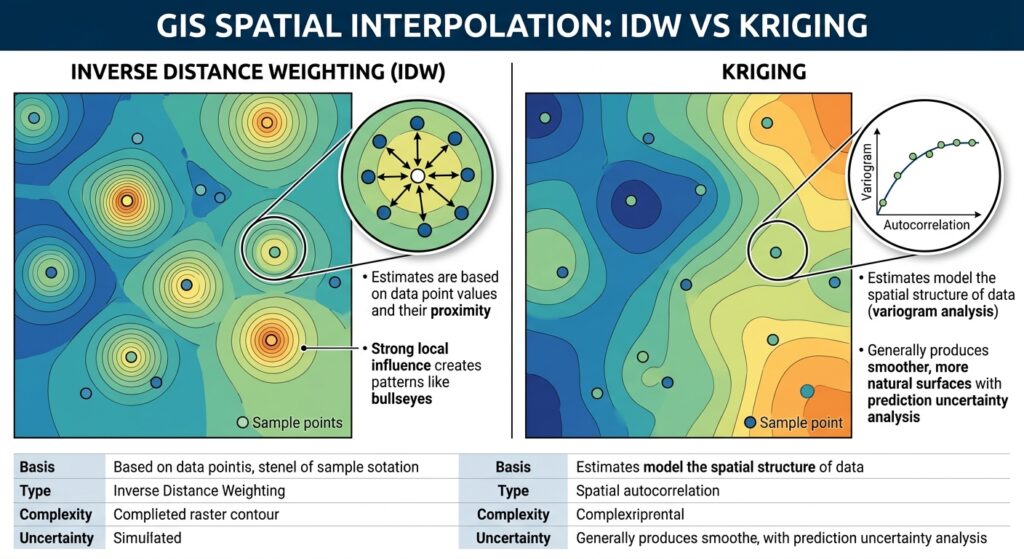
Inverse Distance Weighting (IDW) is a deterministic interpolation method. It assumes that nearby observations have more influence on an unknown location than observations farther away.

The basic idea can be expressed as:

Estimated value = weighted average of nearby sample values

The weights decrease as distance increases:

$wi=1dipw_i = \frac{1}{d_i^p}$

where:

$wiw_i$ = weight assigned to sample point i
$did_i$ = distance between the sample and prediction location
$pp$ = power parameter

A higher power gives nearby points substantially more influence.

For example, with a power of 2, a point twice as far away receives approximately one-quarter of the weight of a nearby point, assuming the other conditions are equal.

What Is Kriging?

Kriging is a geostatistical interpolation method. Unlike basic IDW, it attempts to model the spatial structure of the dataset before generating predictions.

Kriging relies heavily on spatial autocorrelation: the idea that observations located close together tend to have more similar values than observations that are far apart.

A key component is the variogram, which describes how similarity or variability changes with distance.

The variogram helps determine how much influence observations at different distances should have when estimating an unknown location.

IDW vs Kriging at a Glance

Characteristic	IDW	Kriging
Method type	Deterministic	Geostatistical
Main principle	Distance	Spatial autocorrelation
Variogram required	No	Yes
Parameters	Power, search radius/neighbors	Variogram model, range, nugget, sill
Complexity	Relatively simple	More advanced
Produces prediction uncertainty	Generally no	Can produce prediction/error information
Sensitive to clustering	Yes	Can explicitly account for spatial structure
Best starting point	Simple datasets	Data with meaningful spatial autocorrelation

5 Key Differences Between IDW and Kriging

1. Distance vs Spatial Structure

IDW primarily asks:

How far is each sample from the location being predicted?

Kriging asks a more sophisticated question:

How does the variable’s spatial relationship change with distance?

This makes Kriging particularly useful when your dataset has measurable spatial autocorrelation.

2. Parameter Selection

IDW commonly requires you to select a power value, search radius, or number of neighboring points.

Kriging requires decisions about the variogram and its parameters, such as the nugget, sill, range, and model type.

This makes Kriging more demanding for beginners but potentially more statistically defensible.

3. Bullseye Patterns

IDW can create circular “bullseye” patterns around individual sample points.

This happens because the sample point has the greatest influence on nearby predictions, particularly when using a high power value.

Kriging generally produces smoother surfaces when the variogram appropriately represents the underlying spatial structure.

4. Prediction Uncertainty

Kriging can provide information about prediction uncertainty. This is particularly valuable when your assignment requires you to assess where interpolation predictions are more or less reliable.

IDW generally focuses on producing the estimated surface rather than explicitly modeling prediction uncertainty.

5. Computational Complexity

IDW is comparatively straightforward to configure and explain.

Kriging involves more assumptions and requires additional analysis, particularly when selecting and validating the variogram model.

Pro Tip: Don’t automatically assume that Kriging is better simply because it is more sophisticated. For a small, irregularly distributed dataset without clear spatial autocorrelation, a carefully configured IDW surface may be perfectly appropriate.

How to Run IDW Interpolation in QGIS

QGIS provides several interpolation options through its Processing framework, including tools associated with native, SAGA, and GDAL workflows depending on your installation and version.

Step 1: Prepare Your Point Data

Start with a point layer containing your measured variable.

For example:

Station	Rainfall_mm
Station 1	850
Station 2	920
Station 3	780
Station 4	1,050

Make sure the attribute containing the measured values is numeric.

Also check the coordinate reference system (CRS).

Pro Tip: For distance-based interpolation, a projected CRS with appropriate linear units is generally preferable to geographic latitude/longitude coordinates.

Step 2: Open the Interpolation Tool

In QGIS, open:

Processing → Toolbox

Search for IDW or Interpolation.

Depending on your QGIS installation and available providers, the exact tool location and parameters can differ. SAGA-based installations may expose additional interpolation algorithms.

Step 3: Select the Input Layer and Field

Choose your point layer as the input.

Select the field containing the measurement you want to interpolate, such as:

rainfall
temperature
elevation
pollutant concentration
groundwater level

Step 4: Configure the Power Parameter

Set the IDW power.

A common starting value is 2, although the correct value depends on your dataset.

A lower power creates a smoother surface because distant observations retain more influence. A higher power emphasizes nearby observations and can create stronger local variations.

Step 5: Define the Output Extent and Resolution

Set the interpolation extent to cover your study area.

Choose an appropriate raster cell size.

Avoid choosing an extremely small cell size simply because it creates a visually detailed map. The raster resolution should be consistent with your sample density and the scale of the analysis.

Step 6: Run and Inspect the Raster

Run the interpolation and inspect the resulting raster.

Look for:

unexpected extreme values
circular bullseye patterns
sharp transitions
areas far from sample points
edge effects

[IMAGE PLACEHOLDER: QGIS IDW interpolation tool showing point layer, interpolation field, power parameter, extent, and output raster | Alt Text: QGIS IDW interpolation settings for GIS spatial analysis]

How to Run Kriging in QGIS

Kriging workflows in QGIS can vary considerably depending on the installed Processing providers and QGIS version. SAGA provides several geostatistical tools that may be available through the Processing Toolbox.

Step 1: Examine Your Sample Distribution

Before running Kriging, map the sample points.

Check whether the observations appear spatially clustered or whether there is a meaningful spatial pattern.

You should also examine the measured values for obvious outliers.

Step 2: Open the Kriging Tool

Go to:

Processing → Toolbox

Search for Kriging.

If the required SAGA provider is installed and enabled, you may find SAGA Kriging algorithms in the results.

Step 3: Select the Measurement Field

Choose the numerical field you want to predict.

For example, if your layer contains soil samples, you might interpolate:

Soil_Moisture

Step 4: Choose a Variogram Model

Kriging requires a model describing spatial dependence.

Common variogram models include:

Spherical
Exponential
Gaussian

The appropriate model depends on the spatial behavior of your dataset.

For a university assignment, don’t simply select a model without explanation. State which model you used and why it was selected.

Step 5: Configure Neighborhood and Output Settings

Specify the search neighborhood, raster extent, and cell size.

Avoid using too many distant points if the dataset has strong local spatial variation.

Step 6: Generate and Evaluate the Surface

Run the interpolation and inspect the output.

If your workflow provides an associated prediction-error surface, examine that raster as well.

How to Run IDW in ArcGIS Pro

In ArcGIS Pro, IDW is available through the Spatial Analyst extension.

Step 1: Add Your Sample Points

Add the point dataset to your ArcGIS Pro project.

Open the attribute table and confirm that the measurement field contains valid numeric values.

Step 2: Open IDW

Navigate to:

Analysis → Tools

Search for:

IDW

The tool is available under the Spatial Analyst interpolation tools when the appropriate extension is licensed.

Step 3: Set the Input Field

Select your sample point layer.

Set the Z value field to the attribute containing your measurements.

For rainfall, this might be:

Annual_Rainfall

Step 4: Set the Power

Enter an appropriate power value.

Start with a value such as 2 if your assignment does not specify one, then test alternatives where appropriate.

Document the parameter in your methodology.

Step 5: Define Cell Size and Extent

Set the output cell size and processing extent.

Use a study-area boundary where appropriate rather than generating a huge raster outside the region supported by your observations.

Step 6: Run the Tool

Click Run and inspect the resulting raster.

You can use the raster symbology to visualize high and low estimated values.

How to Run Kriging in ArcGIS Pro

ArcGIS Pro provides Kriging through its Geostatistical Analyst capabilities.

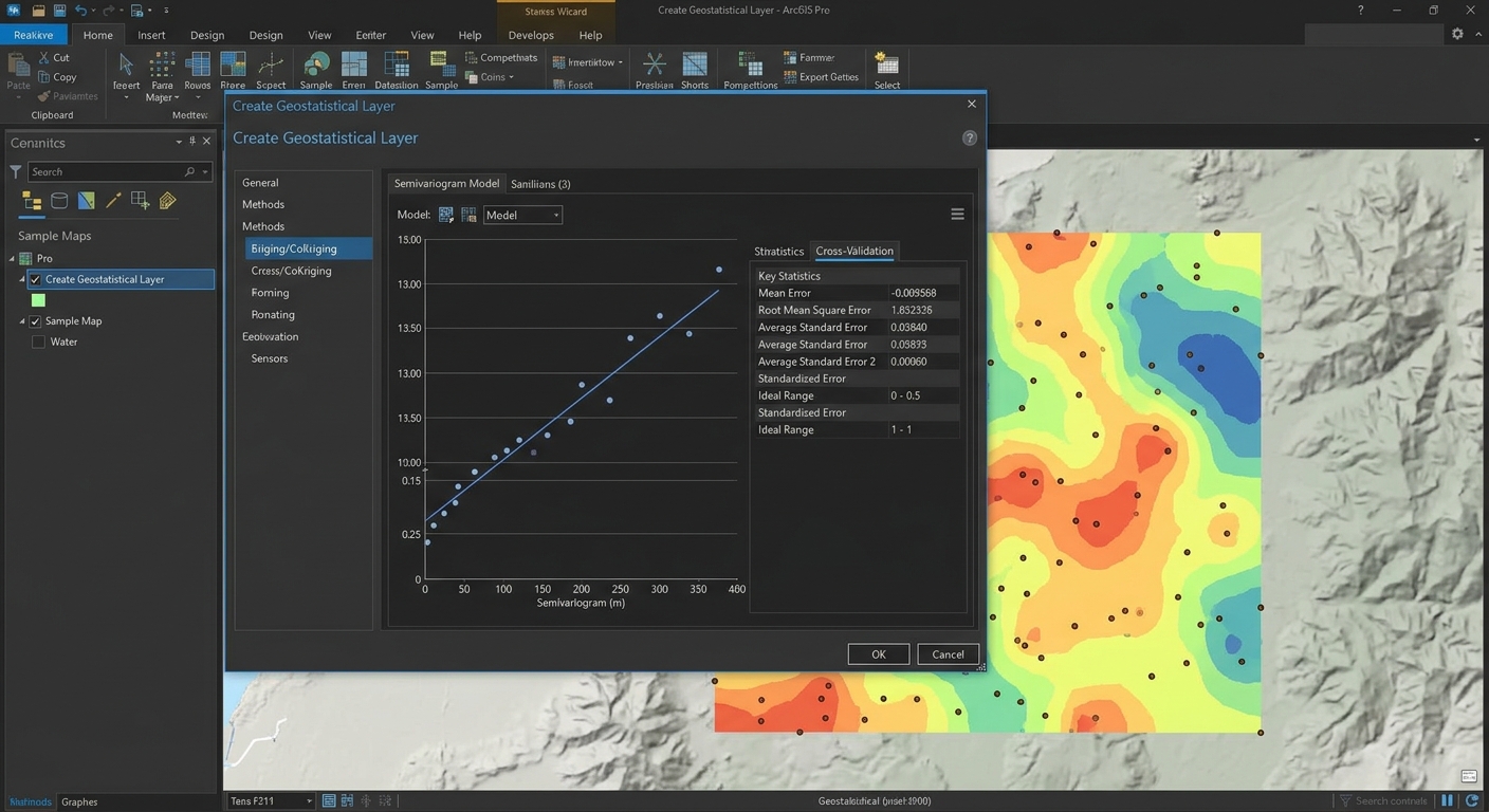
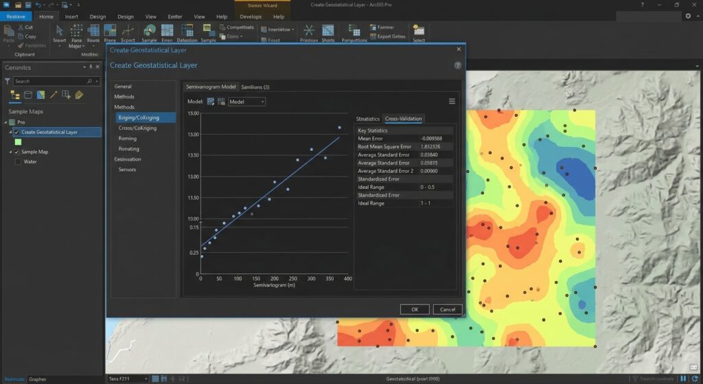
Step 1: Open Geostatistical Wizard

Go to:

Analysis → Geostatistical Wizard

Select your point dataset and measurement field.

Step 2: Select Kriging

Choose an appropriate Kriging method.

Depending on your analysis, options may include ordinary or universal Kriging.

For many introductory assignments, Ordinary Kriging is a logical starting point when the mean is assumed to be relatively constant across the study area.

Step 3: Examine the Semivariogram

The Geostatistical Wizard allows you to examine spatial relationships between sample locations.

Inspect the semivariogram and model fit.

You may compare different models and assess how well they represent the observed spatial structure.

Step 4: Perform Cross-Validation

Use the cross-validation functionality to assess prediction performance.

Important statistics can include:

Mean Error
Root Mean Square Error (RMSE)
Average Standard Error
Standardized statistics

Step 5: Create the Geostatistical Layer

Once the model is satisfactory, generate the geostatistical layer.

You can subsequently export or convert the results into a raster when required by your assignment.

When to Use IDW vs Kriging GIS in Lab Assignments

The best interpolation method depends on the question your assignment is asking.

Choose IDW When:

You need a relatively simple interpolation method.
Your assignment emphasizes deterministic interpolation.
Sample values are strongly influenced by nearby observations.
You have limited statistical information about spatial structure.
You need a quick baseline surface for comparison.

IDW is particularly useful as a baseline model. You can compare its output against a more sophisticated Kriging model.

Choose Kriging When:

Your dataset demonstrates spatial autocorrelation.
You need to model spatial dependence.
Your assignment specifically requires geostatistical analysis.
You need prediction uncertainty.
You have enough observations to support variogram analysis.

If your professor asks you to compare interpolation techniques, running both methods can be more informative than selecting only one.

Pro Tips for Improving Interpolation Accuracy

Pro Tip 1: Check Sample Density

Interpolation cannot create reliable information where there are no supporting observations.

If 90% of your sample points are concentrated in one part of the study area, predictions in sparsely sampled regions should be treated cautiously.

Rule of thumb: More samples generally improve your ability to represent local spatial variation, but simply adding more points does not guarantee accuracy.

Pro Tip 2: Watch Boundary Effects

Interpolation near the edge of your study area can be less reliable because fewer neighboring points may be available.

Avoid interpreting the outermost portions of an interpolation surface without considering the sample distribution.

Pro Tip 3: Don’t Ignore Outliers

An extreme sample value can strongly affect IDW and may also influence Kriging model fitting.

Investigate unusual observations before automatically deleting them.

An outlier may represent an error—or a genuinely important environmental condition.

Pro Tip 4: Use Cross-Validation

If your software supports cross-validation, use it.

RMSE (Root Mean Square Error) is particularly useful because it summarizes the magnitude of prediction errors:

$RMSE=∑(Observed−Predicted)2nRMSE = \sqrt{\frac{\sum (Observed – Predicted)^2}{n}}$

Lower RMSE generally indicates better predictive performance, assuming the models were evaluated using the same observations and validation procedure.

However, don’t choose a method using RMSE alone. Also consider whether the model makes geographical and environmental sense.

Pro Tip 5: Match Resolution to Your Data

A 1-meter raster does not magically make a dataset containing 20 widely spaced samples more accurate.

Raster resolution should reflect the scale of your observations and the purpose of your analysis.

IDW vs Kriging GIS: Which One Should You Choose?

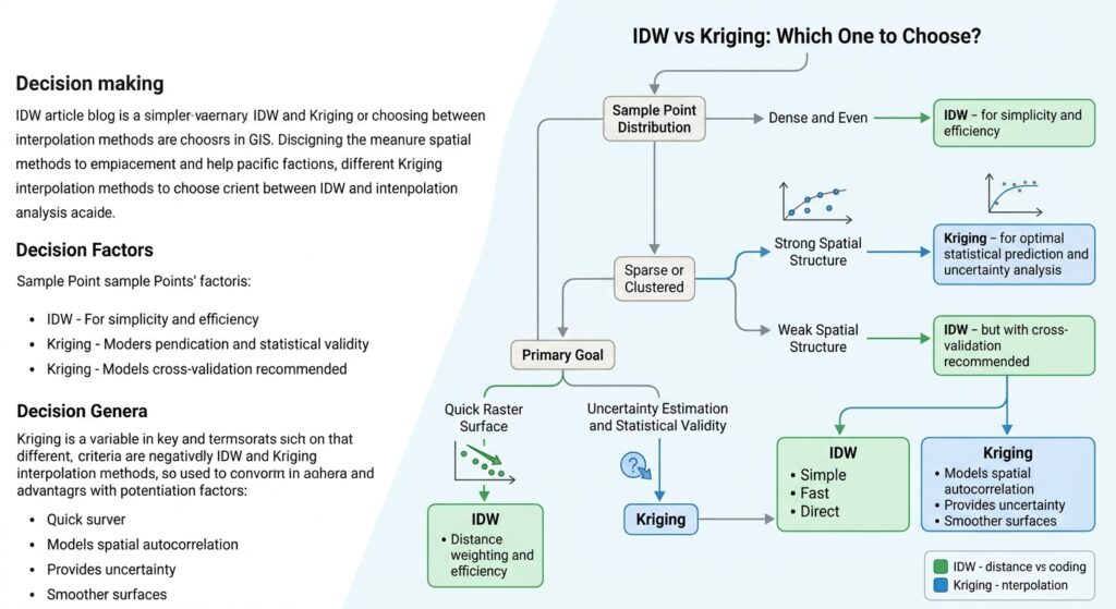
A useful decision process is:

Step 1: Identify the variable.

Is it temperature, rainfall, elevation, pollution, soil moisture, or something else?

Step 2: Examine the sample points.

Are they evenly distributed or heavily clustered?

Step 3: Examine spatial autocorrelation.

If spatial structure is important and can be modeled, Kriging becomes more attractive.

Step 4: Run a baseline IDW model.

This gives you a straightforward reference surface.

Step 5: Run Kriging where appropriate.

Compare the resulting surface and validation statistics.

Step 6: Evaluate accuracy.

Use cross-validation and RMSE where available.

Step 7: Explain your choice.

A strong GIS lab report doesn’t simply say “I selected Kriging because it is more accurate.” Explain how the data structure, interpolation assumptions, parameter settings, and validation results influenced your decision.

Common GIS Interpolation Mistakes

Using Geographic Coordinates for Distance Calculations

If your data is stored in latitude and longitude, distance calculations can be inappropriate for some interpolation workflows.

Consider using an appropriate projected CRS for distance-based analysis.

Using Too High an IDW Power

A very high power can make the output excessively controlled by individual observations.

This can produce sharp local peaks and bullseye patterns.

Treating the Raster as Ground Truth

An interpolated raster is an estimate, not a direct measurement.

Every cell without an observed sample value represents a prediction.

Ignoring the Study Area Boundary

Don’t assume the interpolation surface is equally reliable everywhere. Areas far from sample locations often have greater uncertainty.

Failing to Document Parameters

For your lab report, record:

Input dataset
Measurement field
CRS
Interpolation method
IDW power or Kriging model
Search radius/neighborhood
Cell size
Output extent
Validation method
RMSE or other accuracy statistics

This makes your workflow reproducible.

External Resources for GIS Interpolation

For climate and environmental datasets, students can consult:

Explore [USGS Educational Resources](https://www.usgs.gov/educational-resources) for environmental datasets.

For additional information about geostatistical interpolation:

Refer to the official [Esri Geostatistical Analyst Documentation](https://pro.arcgis.com/en/pro-app/latest/help/analysis/geostatistical-analyst/what-is-geostatistical-analyst-.htm) for advanced Kriging models.

These resources can help you identify suitable datasets and understand the underlying geostatistical concepts before beginning your GIS lab.

Frequently Asked Questions (FAQ)

What is the main difference between deterministic and geostatistical interpolation?

Deterministic methods such as IDW primarily use mathematical relationships such as distance. Geostatistical methods such as Kriging model spatial autocorrelation and use variograms to represent spatial dependence.

Why does IDW produce a “bullseye” effect on interpolated maps?

IDW strongly weights nearby sample points. When an isolated point has a substantially different value, the surrounding cells can form circular zones around it, creating a visible bullseye pattern.

Which method is better for elevation mapping: IDW or Kriging?

Neither is universally better. IDW can work well with dense elevation observations, while Kriging may be preferable when spatial autocorrelation is strong and statistical modeling is required. Compare validation results and terrain characteristics before choosing.

Conclusion: Choosing Between IDW and Kriging

The key to IDW vs Kriging GIS is understanding that the two methods make different assumptions about spatial variation.

IDW is straightforward and distance-driven. It is often an excellent starting point when you need a simple interpolation surface and don’t have enough information to model spatial structure.

Kriging is more sophisticated because it uses spatial autocorrelation and variogram analysis. It can be especially useful when your dataset has a meaningful spatial structure and your assignment requires geostatistical analysis or prediction uncertainty.

For a strong GIS lab submission, don’t simply produce a colorful interpolation map. Explain why you selected the method, how you configured its parameters, where the predictions may be unreliable, and how you evaluated accuracy.

If you’re working on a GIS lab assignment right now, comment with your dataset type, number of sample points, and the variable you’re trying to interpolate, and you can use those details to determine whether IDW or Kriging is the more defensible choice.