
Spatial Join in ArcGIS Pro: A Hands-On Guide for GIS Students
A spatial join in ArcGIS Pro combines information from two datasets based on their geographic relationship rather than a common attribute field. Unlike a traditional attribute join, which connects records using something like Student_ID or County_ID, a spatial join asks questions such as “Which county contains this point?”, “How many schools are inside each district?”, or “What is the nearest hospital to each settlement?”
Spatial joins are particularly useful for point-in-polygon analysis, proximity analysis, and summarizing features within geographic boundaries.
Attribute Join vs Spatial Join
The fundamental difference is how records are matched.
| Join Type | Records are matched using | Example |
|---|---|---|
| Attribute Join | A common field/value | Join population statistics to counties using County_ID |
| Spatial Join | Geographic location | Assign each school the county polygon containing it |
| Distance Spatial Join | Geographic proximity | Find the nearest hospital to every settlement |
Simple example
Suppose you have:
Schools
| School_ID | Name | Location |
|---|---|---|
| S01 | School A | Point |
| S02 | School B | Point |
| S03 | School C | Point |
and:
Counties
| County_ID | County | Geometry |
|---|---|---|
| 001 | County A | Polygon |
| 002 | County B | Polygon |
There may be no common ID connecting the two tables.
A spatial join can determine:
School A → County A
School B → County A
School C → County B
The relationship comes from where the features are located.
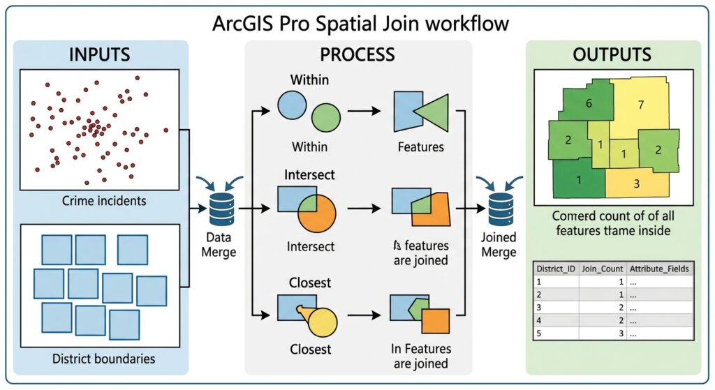
Understanding Target Features and Join Features
One of the most important concepts in ArcGIS Pro is understanding the difference between Target Features and Join Features. Mastering target and join features is critical when performing a spatial join in ArcGIS Pro.
Target Features
The Target Features are the features you want to retain in the output.
Join Features
The Join Features provide information that will be attached to the target features.
Think of it as:
Target = “Who am I adding information to?”
Join = “Where am I getting that information from?”
Example: Schools inside counties
Target Features:
Schools

Join Features:
Counties
The output remains based on the school features, while information from the containing county is added.
Example: Number of schools per county
Reverse the perspective:
Target Features:
Counties

Join Features:
Schools
Now the output is based on counties, and the schools are summarized against them.
This distinction is essential when performing a spatial join target join features workflow.
Spatial Join Match Options
ArcGIS Pro provides several spatial relationships for determining which features should be joined.
The correct option depends on the question you are asking.
1. Intersect
Intersect matches features that share some portion of their geometry. he intersect match option is frequently used during a spatial join in ArcGIS Pro to identify overlapping layers.
For example:
Which roads intersect flood-risk polygons?
If a road crosses a flood-zone polygon, the two features can be considered a spatial match.
Concept
Road
───────────────
       │
       │ Flood Zone
       │ █████
       │ █████
       │
The road and flood polygon share geographic space.
Useful for
- Lines crossing polygons
- Polygons overlapping polygons
- Points falling within polygons
- General spatial relationships
2. Contains
Contains asks whether the target feature completely contains the join feature. When evaluating point-in-polygon relationships, running a spatial join in ArcGIS Pro with the Contains rule isolates features inside boundaries.
For example:
Which county contains each school?
Here:
Target → County
Join   → School
The county contains the school point.
Conceptually:
┌──────────────────────┐
│                      │
│       County         │
│          • School    │
│                      │
└──────────────────────┘
This is particularly useful for point-in-polygon analysis.
3. Within
Within is the reverse spatial relationship.
It asks whether the target feature is located within the join feature.
For example:
Target → School
Join   → County
The school is within the county.
This distinction becomes important when you change the direction of the spatial join.
Practical rule
If you are unsure whether to use Contains or Within, first ask:
Which feature contains which?
Then check which dataset is the target.
4. Closest
Closest matches a target feature with the nearest join feature. Proximity analysis relies heavily on executing a spatial join in ArcGIS Pro with the Closest match setting.
This is particularly useful for distance spatial join analysis.
For example:
Find the nearest hospital to every village.
You might have:
Villages → Target Features
Hospitals → Join Features
ArcGIS Pro can identify the closest hospital for each village.
The resulting table might look like:
| Village | Nearest Hospital | Distance |
|---|---|---|
| Village A | Hospital 3 | 2.4 km |
| Village B | Hospital 1 | 5.1 km |
| Village C | Hospital 2 | 1.7 km |
This type of analysis is useful for:
- Healthcare accessibility
- Emergency planning
- Retail analysis
- Transport studies
- Service-area research
Step-by-Step: Performing a Spatial Join in ArcGIS Pro
Let’s use a practical university GIS example:
Determine how many schools are located within each administrative district.
We have:
Districts → Polygon layer
Schools   → Point layer
We want the final output to contain the districts plus a count of schools inside each district.
Step 1: Prepare Your Data
Open your ArcGIS Pro project and add both layers.
For example:
Administrative_Districts
Schools
Check that both datasets:
- Are correctly positioned
- Use appropriate coordinate systems
- Have valid geometries
- Cover the same study area
[Insert Screenshot of ArcGIS Pro Map Showing District Polygons and School Points]
Step 2: Open the Spatial Join Tool
Locate and launch the spatial join in ArcGIS Pro tool from the Geoprocessing pane.
Open the Geoprocessing pane.
Search for:
Spatial Join
Open:
Analysis → Tools → Spatial Join
The tool contains several important parameters.
[Insert Screenshot of Spatial Join Pane]
Step 3: Set Target Features and Join Features
For our example:
Target Features:
Administrative_Districts

Join Features:
Schools
This tells ArcGIS Pro:
Keep the district polygons and attach information about the schools located within them.
Why this direction matters
If you reverse the layers:
Target:
Schools

Join:
Administrative_Districts
you would instead produce a school-based output where each school receives information about its containing district.
Neither approach is inherently wrong—the correct setup depends on the question being answered.
Step 4: Choose the Join Operation
ArcGIS Pro provides two important options:
One-to-One
A single target feature produces one output record.
For our example:
District A → 15 schools
District B → 22 schools
District C → 8 schools
Each district remains one record.
This is ideal when you want to summarize join features.
One-to-Many
A target feature can produce multiple output records when multiple join features match it.
For example:
District A
    ↓
School 1
School 2
School 3
The resulting output contains separate relationships between the target and matching join features.
When to use each
| Join Operation | Output behavior | Typical use |
|---|---|---|
| One-to-One | One record per target | Count schools per district |
| One-to-Many | Multiple records for multiple matches | Preserve individual school-to-district relationships |
For most summary analyses, One-to-One is the more appropriate choice.
Step 5: Choose the Match Option
For our school-count example, choose the spatial relationship that identifies schools located inside districts.
Depending on the direction and geometry relationship, use the appropriate containment/intersection relationship.
For example:
Match Option:
Contains / Within
The important point is to verify the relationship against your target and join direction rather than selecting the option mechanically.
Step 6: Configure the Field Map
The Field Map controls how attributes from the join features are transferred or summarized. Setting up field map merge rules ensures your spatial join in ArcGIS Pro aggregates numeric fields accurately.
This becomes particularly important when several schools match one district.
[Insert Screenshot of Field Map Settings in ArcGIS Pro]
Suppose the school layer contains:
School_ID
School_Name
Enrollment
School_Type
You might want to calculate:
- Number of schools
- Total enrollment
- Average enrollment
Count
A Count merge rule can be used to determine how many matching records exist.
For example:
District A → 15
District B → 22
District C → 8
The resulting field might be called:
School_CountThis is the classic spatial join count field workflow.
Using Sum
Suppose each school has an Enrollment field:
| School | Enrollment |
|---|---|
| School A | 450 |
| School B | 300 |
| School C | 650 |
You can use the Sum merge rule to calculate total enrollment within each district.
For example:
District A
450 + 300 + 650
= 1,400 students
The output could contain:
| District | School_Count | Total_Enrollment |
|---|---|---|
| District A | 3 | 1,400 |
Using Mean
The Mean merge rule calculates the average value of a numeric field among matching features.
For example:
School enrollment:
450
300
650

Mean = 466.7
This can be useful when investigating:
- Average school enrollment
- Average property value
- Average elevation
- Average household size
Make sure the field is appropriate for mathematical aggregation.
Step 7: Run the Spatial Join
Specify an output feature class, such as:
Districts_School_CountReview your settings:
Target:
Administrative_Districts

Join:
Schools

Join Operation:
One-to-One

Match Option:
Appropriate containment relationship

Output:
Districts_School_Count
Click Run.
Step 8: Examine the Output
Add the resulting layer to your map.
Open its attribute table.
You should now have something similar to:
| District | School_Count | Total_Enrollment |
|---|---|---|
| District A | 15 | 8,420 |
| District B | 22 | 11,240 |
| District C | 8 | 3,670 |
The spatial join has transformed the original point dataset into useful information about the polygon dataset.
Example 2: Point-in-Polygon Spatial Join
Crime analysis often requires a spatial join in ArcGIS Pro to count incidents within ward boundaries.
Suppose you have:
- 2,000 crime locations
- 20 administrative wards
Your research question is:
How many reported incidents occurred in each ward?
Set:
Target:
Wards

Join:
Crime_Points

Join Operation:
One-to-One
Use the appropriate point-in-polygon spatial relationship.
The resulting Join_Count or equivalent count field tells you how many crime points were matched to each ward.
This is one of the most common undergraduate GIS spatial-analysis workflows.
Example 3: Distance Spatial Join
Now consider a different question:
What is the nearest health facility to every settlement?
Use:
Target:
Settlements

Join:
Health_Facilities
Choose:
Match Option:
Closest
Where supported by the workflow, specify an appropriate search radius or distance constraint.
The output can include information about the nearest facility and its distance from the target feature.
Example output
| Settlement | Facility | Distance |
|---|---|---|
| A | Health Centre 1 | 1.8 km |
| B | Hospital 3 | 4.2 km |
| C | Clinic 2 | 0.9 km |
This is a basic form of proximity analysis.
Common Mistakes and Troubleshooting
Mismatched coordinate systems can cause your spatial join in ArcGIS Pro to yield zero matches.
1. The Join Count Is Zero
If you expected matches but every feature has a count of zero, check:
First: Are the layers actually overlapping?
Zoom to the datasets and inspect them visually.
Second: Is the match relationship correct?
A common mistake is reversing the target and join features or choosing the wrong spatial relationship.
Third: Check the CRS
Two layers can appear incorrectly positioned if their coordinate systems are incorrectly defined.
Fourth: Check the data geometry
Invalid geometries can interfere with spatial relationships.
2. Wrong Target and Join Direction
This is probably the most common conceptual mistake.
Suppose the question is:
“How many schools are in each county?”
Correct conceptual setup:
Target = Counties
Join   = Schools
But if the question is:
“Which county is each school located in?”
then:
Target = Schools
Join   = Counties
Always write the research question first.
Then determine which features need to remain as the output.
3. Memory Errors with Large Spatial Joins
Spatial joins can become computationally expensive when working with very large datasets.
For example:
- Millions of points
- Very detailed polygons
- Large raster-derived vector datasets
- Nationwide datasets
Possible solutions include:
Reduce unnecessary features
Clip both datasets to your study area before performing the join.
Simplify unnecessarily complex geometry
Extremely detailed polygons can increase processing requirements.
Use an appropriate spatial index
Many modern GIS formats and geoprocessing workflows use spatial indexing to speed up spatial searches.
Process in smaller geographic units
For very large datasets, consider dividing the study area into manageable regions and processing them separately where appropriate.
4. Wrong Spatial Reference Warnings
A spatial join depends on accurate spatial positioning.
Check:
Layer CRS
    ↓
Project CRS
    ↓
Spatial alignment
Do not confuse:
Defining a projection
with:
Reprojecting data.
If a dataset has an incorrect CRS definition, assigning the correct definition is different from converting it into another CRS.
For distance analysis, also consider whether the coordinate system is appropriate for the units and accuracy you need.
5. Using Closest Without Thinking About Distance
A nearest-feature match always gives you a nearest feature if the search conditions allow one.
That does not necessarily mean the result is practically meaningful.
For example:
Village
   •
   |
   | 75 km
   |
Hospital
The hospital may technically be the closest, but 75 km could be an important finding rather than a convenient service relationship.
For research, consider establishing a meaningful distance threshold.
6. Unexpected Duplicate Records
If you choose One-to-Many, a single target feature can appear in multiple output records.
For example:
County A → School 1
County A → School 2
County A → School 3
This is expected behavior.
If your assignment requires one row per county, use One-to-One and an appropriate field aggregation method.
Spatial Join Decision Guide
Use this quick decision process before running the tool:
What is my research question?
             ↓
What features should remain in the output?
             ↓
        TARGET FEATURES
             ↓
What features provide information?
             ↓
         JOIN FEATURES
             ↓
How should they relate?
             ↓
 ┌───────────┼────────────┐
 ↓           ↓            ↓
Within    Intersect    Closest
 ↓           ↓            ↓
Contain-   Shared      Nearest
ment       space       feature
             ↓
How should multiple matches be handled?
             ↓
     One-to-One / One-to-Many
             ↓
How should numeric attributes be summarized?
             ↓
 Count / Sum / Mean / other rule
Quick Reference Table
| Goal | Target | Join | Match concept | Recommended output |
|---|---|---|---|---|
| Assign county to every school | Schools | Counties | Within/Contains relationship | One-to-One |
| Count schools per county | Counties | Schools | Point-in-polygon | One-to-One + Count |
| Preserve every school relationship | Counties | Schools | Point-in-polygon | One-to-Many |
| Calculate total enrollment per county | Counties | Schools | Point-in-polygon | One-to-One + Sum |
| Calculate average enrollment | Counties | Schools | Point-in-polygon | One-to-One + Mean |
| Find nearest hospital | Settlements | Hospitals | Closest | One-to-One |
| Find nearby features within a specified distance | Target layer | Nearby features | Distance-based match | Depends on study design |
Final Takeaway
The key to performing a successful spatial join in ArcGIS Pro is to think about the analysis before opening the tool.
Remember:
Target Features = the features you want to keep.
Join Features = the features providing information.
Then determine the spatial relationship—such as Intersect, Contains, Within, or Closest—and decide whether your analysis requires One-to-One or One-to-Many output.
For quantitative analysis, the Field Map is equally important because merge rules such as Count, Sum, and Mean determine how multiple matching features are summarized. Finally, always check CRS, geometry, feature counts, and the resulting attributes before treating the spatial join as a finished analytical result.