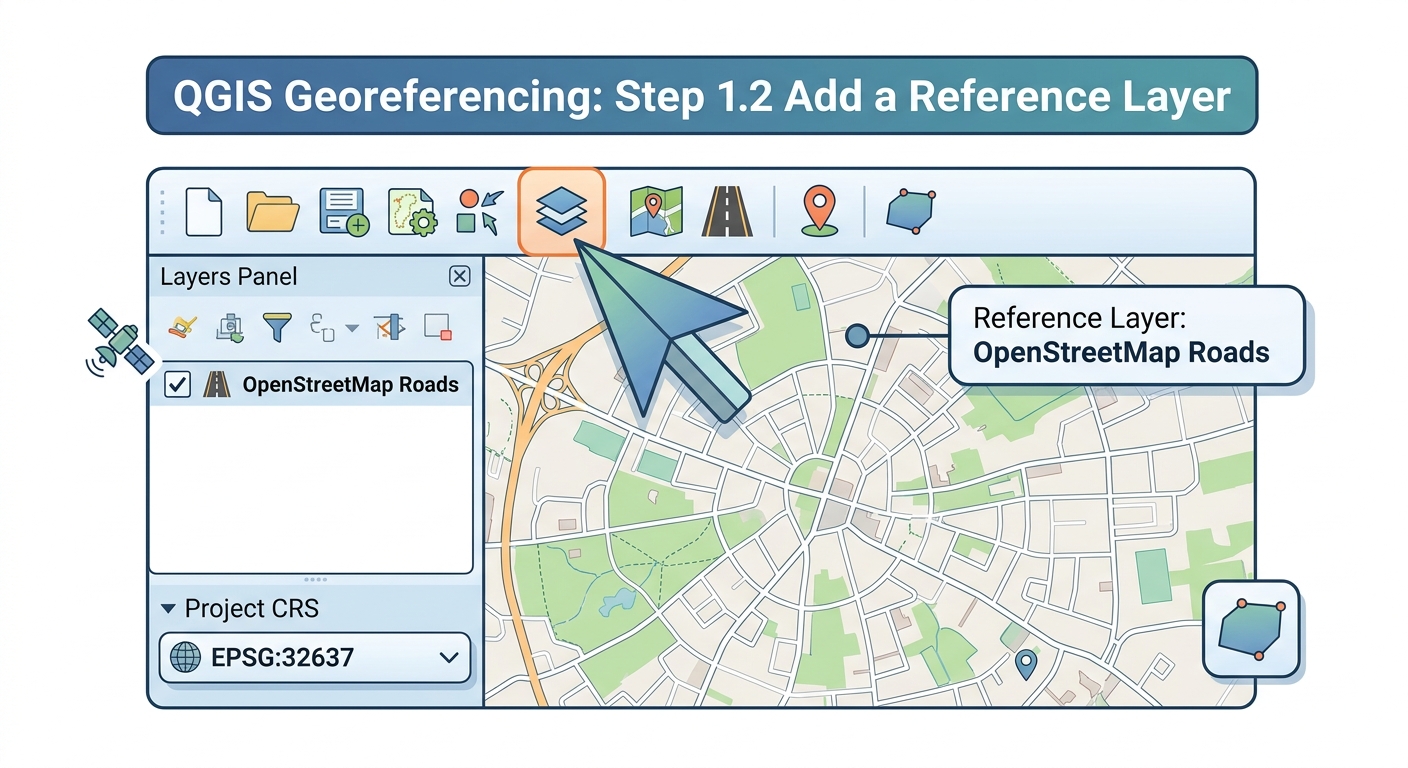
How to Georeference an Image in QGIS: A Complete Step-by-Step Workflow

Georeferencing assigns real-world geographic coordinates to an image that does not already contain spatial reference information. In this guide, you will learn how to georeference an image in QGIS using a scanned historical map, CAD print, aerial photograph, or other unreferenced raster. The process uses identifiable ground control points (GCPs), a coordinate reference system (CRS), and a spatial transformation to align the image with modern geographic data.

Georeferencing is particularly useful when working with historical maps because the original map may show roads, rivers, boundaries, or settlements without storing their modern geographic coordinates.

---

What You Need Before Starting

Before diving into how to georeference an image in qgis, gather your scanned rasters and reference basemaps.

For this workflow, prepare:

• An unreferenced scanned map, preferably PNG, JPG, or TIFF
• A QGIS project
• A reference layer or basemap with known geographic coordinates
• Several identifiable control points
• An appropriate CRS for the study area

Good control points might include:

• Road intersections
• Bridges
• Building corners
• River junctions
• Church or railway locations
• Survey monuments
• Clearly identifiable coastline features

For historical maps, choose features that have not moved significantly over time.

---

Step 1: Load the Basemap and Set the Project CRS

The first step is to establish a spatial reference framework for the map you are going to georeference. Setting up your reference layer correctly is foundational when learning how to georeference an image in qgis. Matching your reference layer’s spatial parameters is crucial when learning how to georeference an image in qgis effectively.

1.1 Open QGIS

Start a new QGIS project.

Open:

Project → New

Save the project before beginning.

A useful project structure might be:

Historical_Map_Project/
│
├── raw/
│   └── historical_map.jpg
│
├── reference/
│   └── roads.gpkg
│
├── output/
│   └── historical_map_georeferenced.tif
│
└── qgis_project/

Keeping the original scan separate from the processed output makes it easier to reproduce your workflow.

---

1.2 Add a reference layer

Load a spatial dataset that already has a valid CRS.

For example:

• OpenStreetMap-derived roads
• Administrative boundaries
• Recent satellite imagery
• Survey data
• Existing GIS vector layers

Use:

Layer → Add Layer

Then select your reference dataset.

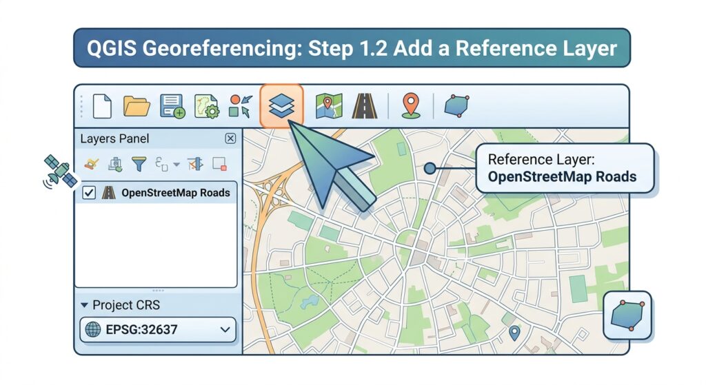
Your reference layer provides the geographic framework against which the scanned map will be aligned.

---

1.3 Set the project CRS

Check the CRS displayed in the lower-right corner of the QGIS window.

Click the CRS indicator and select the appropriate coordinate reference system.

For example:

Project CRS:
EPSG:32637 — WGS 84 / UTM zone 37N

The correct CRS depends on your study area and the coordinate system used by your reference data.

Important distinction

The project CRS is not necessarily the same thing as the historical map’s original CRS.

An old map may have been produced using:

• A local grid
• A national coordinate system
• A historical datum
• A paper map with no usable coordinate information

If the original coordinate system is unknown, you can georeference it using identifiable points from a modern reference dataset.

---

Step 2: Launch the Georeferencer and Select Ground Control Points

QGIS includes a dedicated Georeferencer for assigning geographic coordinates to raster images. When learning how to georeference an image in qgis, selecting reliable ground control points is the most critical step. Understanding where to locate toolbar panels streamlines the overall workflow of how to georeference an image in qgis.

Open it from:

Layer → Georeferencer

Depending on your QGIS version, it may appear as:

Layer → Georeferencer → Georeferencer

or through the Raster menu.

---

2.1 Load the scanned map

Inside the Georeferencer window, open your scanned image.

For example:

historical_map.jpg

[Insert Screenshot of QGIS Georeferencer with Historical Map Loaded]

The image will initially have no meaningful geographic position.

Your task is to establish a mathematical relationship between:

Image coordinates → Real-world coordinates

---

What Are Ground Control Points?

A ground control point (GCP) is a recognizable location that can be identified both:

1. On the unreferenced image, and
2. On a geographically referenced dataset.

For example, suppose a historical map contains a distinctive road intersection.

You can click that intersection on the historical map and tell QGIS its corresponding real-world location.

Conceptually:

Historical image
       ↓
   Road junction
       ↓
      GCP
       ↓
Known geographic coordinate
       ↓
Reference map

Several GCPs are needed to establish a reliable transformation.

---

2.2 Choosing good GCPs

Good GCPs should be:

• Clearly identifiable
• Distributed across the entire map
• Stable through time
• Easy to locate precisely
• Ideally located near the edges as well as the center

Avoid putting all your points in one small area.

Poor distribution

┌─────────────────────────────┐
│                             │
│                             │
│       • • • •               │
│       • • • •               │
│                             │
└─────────────────────────────┘

Better distribution

┌─────────────────────────────┐
│ •                         • │
│                             │
│                             │
│          •      •           │
│                             │
│ •                         • │
└─────────────────────────────┘

A well-distributed set of GCPs helps the transformation model work across the entire raster rather than only in one region.

---

2.3 Add your first GCP

Select the Add Point tool in the Georeferencer.

Click a recognizable location on the scanned map.

QGIS will ask you to enter the corresponding geographic coordinate.

Alternatively, if the reference layer is visible in the main QGIS window, you can obtain the coordinate from the reference dataset.

[Insert Screenshot of Adding GCPs in QGIS Georeferencer]

Record the point in the GCP table.

A typical table might look like:

ID	Image X	Image Y	Map X	Map Y
GCP 1	245.2	183.7	36.8219	-1.2921
GCP 2	732.5	191.4	36.8512	-1.2875
GCP 3	238.7	614.9	36.8194	-1.3267
GCP 4	745.1	623.3	36.8531	-1.3214

The exact values will depend on your map and CRS.

---

2.4 Add additional GCPs

Repeat the process for additional recognizable features.

For a simple transformation, use more GCPs than the mathematical minimum.

For example, a first-order polynomial requires at least three non-collinear points, but using only three points leaves little room to identify errors.

A practical student workflow might use:

6–10 well-distributed GCPs

rather than relying on the minimum.

---

Step 3: Choose Transformation Settings and Understand RMS Error

Once your GCPs are established, configure the transformation.

Open the transformation settings in the Georeferencer.

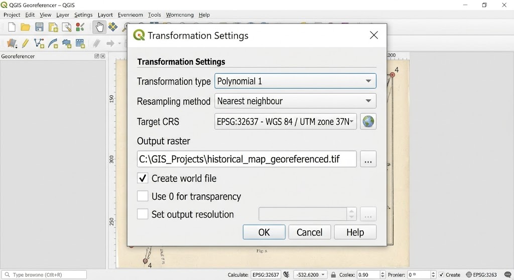
Important settings include:

• Transformation type
• Resampling method
• Target CRS
• Output raster
• Output format
• GCP options

---

Polynomial 1 vs Thin Plate Spline

The transformation model determines how QGIS converts the original image coordinates into geographic coordinates A common question when studying how to georeference an image in qgis is whether to use Polynomial 1 or Thin Plate Spline.

Polynomial 1

A first-order polynomial transformation is often appropriate when the scanned map mainly needs:

• Translation
• Rotation
• Scaling
• Skewing

It treats the transformation relatively simply.

Conceptually:

Original image
      ↓
Scale + Rotate + Shift
      ↓
Georeferenced image

This is often a sensible starting point for a scanned map that has not suffered significant physical deformation.

Use Polynomial 1 when:

• The map is relatively rigid.
• Distortion is limited.
• The map has a consistent scale.
• You want a relatively simple transformation.

---

Thin Plate Spline

Thin Plate Spline (TPS) is a more flexible transformation.

It can accommodate local distortions that a simple polynomial transformation cannot model effectively.

This can be useful for historical maps that have:

• Paper stretching
• Folding
• Local deformation
• Uneven scanning
• Other spatial distortions

Conceptually:

Historical map
~~~~~~~~~~~~~~
  irregular shape
       ↓
Thin Plate Spline
       ↓
Flexible geographic alignment

However, flexibility is not automatically better.

A highly flexible transformation can produce unexpected local distortions if your GCPs are inaccurate or poorly distributed.

---

Understanding RMS Error

The RMS (Root Mean Square) error provides a numerical measure of how closely the transformation fits your control points.

A simplified interpretation is:

How far, on average, the transformed GCP locations differ from their target positions according to the transformation model.

A lower RMS error generally indicates a closer mathematical fit to the selected control points.

However:

A low RMS error does not automatically mean the georeferencing is geographically correct.

For example, if several GCPs were incorrectly identified but consistently placed in the wrong locations, the transformation can still produce an apparently good numerical fit.

Therefore, evaluate:

1. RMS error
2. GCP placement
3. GCP distribution
4. Visual alignment with independent reference data

---

Don’t blindly minimize RMS error

Suppose you have:

GCP 1 → 0.8
GCP 2 → 1.1
GCP 3 → 0.7
GCP 4 → 12.5

The fourth point deserves investigation.

It could represent:

• An incorrectly clicked location
• A feature that changed position
• A coordinate-entry mistake
• A poor-quality reference point
• Genuine historical map distortion

Don’t automatically delete the point simply because it increases RMS error.

First determine why it differs.

---

Step 4: Generate and Verify the GeoTIFF

Once the transformation settings and GCPs are satisfactory, specify the output file.

A recommended output format is GeoTIFF (.tif) because it can store geographic referencing information alongside the raster data.

For example:

historical_map_georeferenced.tif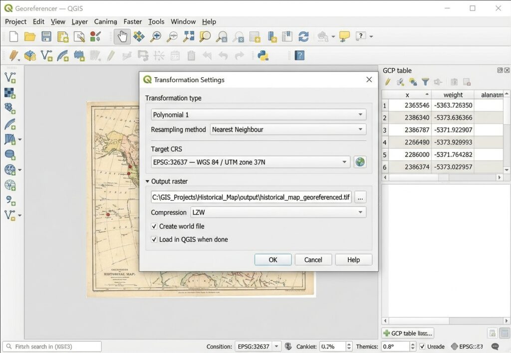 + Add Category 

 

Set the appropriate target CRS.

Then start the georeferencing process.

QGIS will create the transformed raster. Selecting the correct transformation algorithm ensures high geometric precision throughout your how to georeference an image in qgis workflow.

---

4.1 Load the output into QGIS

Add the resulting GeoTIFF to your main QGIS project.

You should now see the historical map positioned geographically.

For example:

Modern reference layer
────────────────────────────

     Roads
       │
   ────┼────────
       │
Historical map
████████████████
████████████████

The historical map should align with recognizable features in your reference data.

---

4.2 Verify alignment visually

Zoom into several locations.

Don’t inspect only the center of the map.

Check:

Center

Does the historical feature align with the modern feature?

Edges

Does the alignment remain reasonable near the map boundaries?

Corners

Do features near the corners remain geographically plausible?

Independent features

Where possible, check features that were not used as GCPs.

This is particularly important because evaluating the same points used to calculate the transformation can give an overly optimistic impression of accuracy.

---

Troubleshooting Common Georeferencing Problems

Problem 1: RMS Error Is Too High

A high RMS error can result from several causes. Managing root mean square (RMS) error values resolves common spatial alignment issues when practicing how to georeference an image in qgis.

Check your GCPs

Look for:

• Incorrect coordinates
• Misidentified features
• Points clicked too far from the actual feature
• Features that changed location
• Poor point distribution

Start by checking the GCP with the largest residual error.

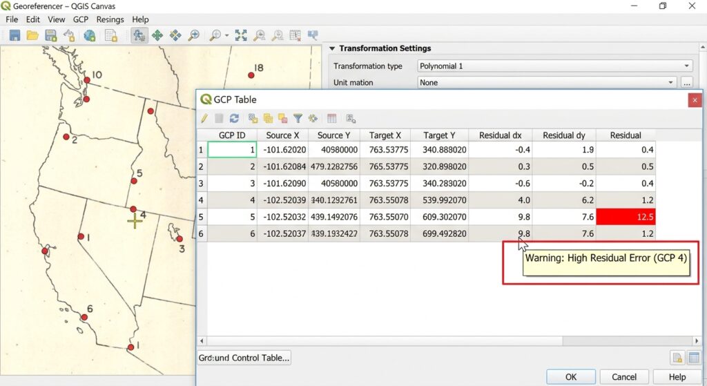
If you discover that the point was incorrectly placed, correct it and recalculate the transformation.

---

Problem 2: The Map Is Correct in the Center but Wrong at the Edges

This often indicates that the selected transformation does not adequately represent the raster’s spatial distortion.

Possible causes include:

• Insufficient GCPs
• Poor GCP distribution
• Map stretching
• Historical paper deformation
• An unsuitable transformation model

Try adding well-distributed GCPs near the problematic areas.

You can also compare a first-order polynomial with a more flexible transformation such as Thin Plate Spline.

---

Problem 3: The Entire Map Is Shifted

If the map has approximately the correct shape but is consistently displaced, check:

• Target CRS
• Coordinate values
• Reference layer CRS
• Project CRS
• GCP coordinate entry

A CRS mismatch can produce a large positional displacement even when the image itself is perfectly fine.

---

Problem 4: The Raster Is Severely Warped

If the output looks dramatically distorted:

1. Check for incorrectly positioned GCPs.
2. Check whether GCPs are concentrated in one area.
3. Reduce unnecessary transformation complexity.
4. Try Polynomial 1 as a baseline.
5. Verify that the target CRS is appropriate.
6. Check whether historical features have changed position.

Do not assume that Thin Plate Spline will automatically fix a poorly controlled dataset.

---

Problem 5: Control Points Are in the Wrong Places

A misplaced GCP can have a significant effect on the transformation.

For example, suppose the actual road intersection is:

        │
────────┼────────
        │

but the GCP is placed several pixels away:

        │
────•───┼────────
        │

The transformation receives incorrect information about the relationship between image and geographic coordinates.

Solution

Zoom in before placing the GCP.

For small features, use a high magnification level so you can click as close as possible to the exact location.

---

Problem 6: Historical Features Have Changed

This is especially important when georeferencing historical maps.

A road intersection, river channel, shoreline, or building may have changed since the map was produced.

For example:

Historical map:

River
~~~~~~~
     \
      \

Modern map:

River
~~~~~~
      \
       \

If you use the modern river location as a GCP for a historical river that has migrated, you introduce an error into the transformation.

Whenever possible, choose stable landmarks.Mastering how to georeference an image in qgis ensures accurate spatial alignment for unreferenced historical maps.

---

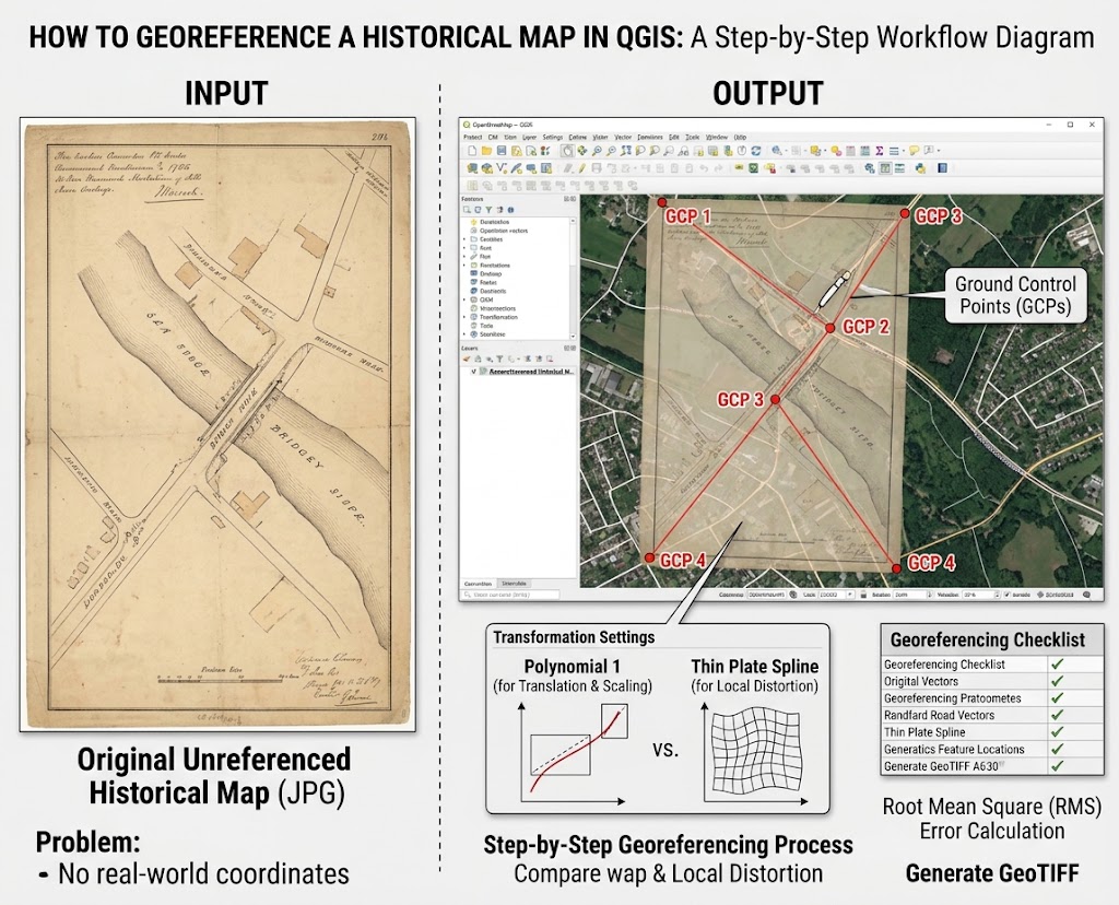
Recommended GCP Strategy

For a student historical-map project, use a workflow such as:

1. Identify stable features
          ↓
2. Distribute GCPs across the map
          ↓
3. Add 6–10+ GCPs
          ↓
4. Start with Polynomial 1
          ↓
5. Inspect RMS/residuals
          ↓
6. Correct obvious GCP errors
          ↓
7. Compare alternative transformations if necessary
          ↓
8. Export GeoTIFF
          ↓
9. Validate against independent reference features

The exact number of GCPs should depend on the map, transformation model, spatial distortion, and intended accuracy.

---

Georeferencing Checklist

Before submitting your GIS assignment or research dataset, check:

Check	Question
Reference CRS	Is the target CRS correct?
GCP quality	Are the points clearly identifiable?
GCP distribution	Are they spread across the entire map?
GCP accuracy	Were points placed precisely?
Transformation	Is the selected model appropriate?
RMS error	Are unusually large residuals investigated?
Visual alignment	Does the map align with independent reference data?
Output	Was the result saved as a GeoTIFF?
Metadata	Have CRS, GCPs, transformation, and source information been documented?

---

Quick Reference: Historical Map Georeferencing in QGIS

️ Image → GCPs → Transformation → GeoTIFF → Validation

1. Load reference data
Establish the geographic framework and appropriate CRS.

2. Open Georeferencer
Load the scanned historical map.

3. Add GCPs
Match recognizable locations on the scan to known geographic coordinates.

4. Choose transformation
Start with Polynomial 1 for relatively rigid maps; consider Thin Plate Spline for genuine local deformation.

5. Evaluate RMS error
Investigate large residuals rather than simply trying to minimize the number.

6. Generate GeoTIFF
Save the transformed raster with its spatial reference information.

7. Validate
Compare the result against independent reference features across the entire map.

Key principle: A low RMS error is useful, but accurate GCP identification, good spatial distribution, an appropriate transformation, and independent visual validation are equally important.

Georeferencing is therefore not simply a matter of making an old map “fit” a modern basemap. It is a spatial transformation process in which the quality of the final dataset depends heavily on the quality and distribution of the ground control points, the chosen transformation model, and the validation procedure.