Table of Contents

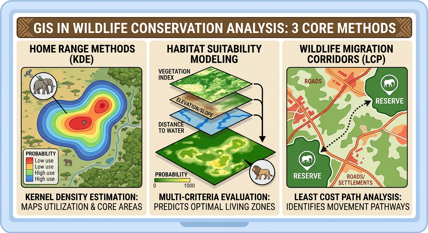
GIS in Wildlife Conservation Analysis: A Practical Guide to Home Range Methods

Wildlife conservation increasingly depends on understanding where animals move, where suitable habitat occurs, and how landscapes connect or fragment those habitats. Geographic Information Systems (GIS) provides the spatial framework for combining wildlife tracking data with satellite imagery, land-cover maps, terrain models, roads, rivers, settlements, and other environmental variables.

GIS in wildlife conservation analysis allows conservationists to move beyond simply recording animal locations. Spatial analysis can estimate an animal’s home range, identify areas with high concentrations of activity, model habitat suitability, and locate potential movement corridors between fragmented habitats.

For ecology and GIS students, three techniques are particularly important:

Home range analysis using Kernel Density Estimation (KDE) and Minimum Convex Polygon (MCP).
Habitat suitability modeling using Multi-Criteria Evaluation (MCE) and raster overlays.
Wildlife corridor mapping using Least Cost Path analysis.

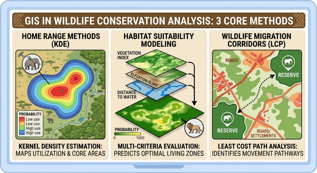
1. 1. GIS in Wildlife Conservation Analysis: Home Range Methods

A home range is the area an animal normally uses d1. GIS in Wildlife Conservation Analysis: Home Range Methodsuring its daily or seasonal activities. Mapping home ranges can help researchers understand feeding areas, resting sites, breeding territories, and responses to habitat disturbance.

GPS collars, radio telemetry, camera traps, or other tracking systems can provide the point locations needed for GIS analysis.

Two commonly used approaches are Minimum Convex Polygon (MCP) and Kernel Density Estimation (KDE).

Minimum Convex Polygon (MCP)

MCP creates the smallest convex polygon containing a specified proportion of an animal’s recorded locations. When applying GIS in wildlife conservation analysis, Minimum Convex Polygon (MCP) offers a quick baseline for estimating home ranges.

For example, a researcher may use 95% of GPS locations to estimate the animal’s overall home range.

The workflow is approximately:

GPS animal locations
        ↓
Check coordinate system and clean data
        ↓
Select tracking locations
        ↓
Calculate Minimum Convex Polygon
        ↓
Calculate polygon area
        ↓
Compare home ranges between animals/seasons

MCP is straightforward and easy to interpret, which makes it useful for introductory wildlife GIS studies.

However, MCP has an important limitation: it assumes the entire polygon represents usable space. An animal may have GPS points on opposite sides of a lake, road, or unsuitable habitat, causing the polygon to include large areas the animal never actually uses.

Kernel Density Estimation (KDE)

Kernel Density Estimation provides a more flexible representation of animal space use.

Instead of drawing a single polygon around all locations, KDE estimates the density of observations across the landscape. Areas containing many tracking points receive higher estimated utilization density.

The result can be displayed as a continuous raster surface:

Low utilization ───────────────► High utilization

This is particularly useful for identifying core-use areas.

For example, a researcher might calculate:

95% KDE → broad home range
50% KDE → core-use area

The exact percentage and bandwidth should be justified according to the study design rather than treated as universal standards.

KDE workflow in GIS

Import GPS tracking points.
Verify the coordinate reference system.
Remove obvious GPS errors and duplicate/problematic observations.
Select an appropriate temporal period.
Calculate the kernel density surface.
Convert density contours into polygons if required.
Calculate the area of the selected utilization contours.
Compare home ranges between individuals, seasons, or years.

Why KDE can be useful

KDE can reveal spatial patterns that MCP hides. Two animals could have similarly sized MCP home ranges while having very different concentrations of activity within those ranges.

2. Habitat Suitability Modeling: GIS in Wildlife Conservation Analysis

Knowing where an animal moves does not necessarily tell us why it uses particular locations.

Habitat suitability modeling addresses this question by combining environmental variables that may influence species occurrence or habitat quality.

A typical model might include:

Land-cover type
Distance to water
Elevation
Slope
Distance from roads
Distance from settlements
Vegetation condition
Human disturbance

These variables can be transformed into comparable suitability scores and combined using Multi-Criteria Evaluation (MCE).

Basic MCE Concept

Habitat suitability modeling is a cornerstone of GIS in wildlife conservation analysis, allowing researchers to combine environmental variables like elevation and land cover.

Suppose an elephant habitat model uses four criteria:

Criterion	Example suitability relationship
Distance to water	Closer = more suitable
Vegetation	More suitable vegetation = higher score
Distance from roads	Farther = potentially more suitable
Slope	Moderate/low slope = potentially more suitable

Each raster is standardized to a common scale, such as:

0 = unsuitable
1 = highly suitable

The standardized layers can then be combined using weighted overlay.

A simplified weighted model could be represented as:

$Suitability=w1X1+w2X2+w3X3+w4X4Suitability = w_1X_1+w_2X_2+w_3X_3+w_4X_4$

where:

$XX$ = standardized environmental criterion
$ww$ = weight assigned to that criterion

The weights should come from a defensible methodology, such as ecological literature, expert elicitation, field evidence, or statistical modeling.

Raster Overlay Workflow

A typical QGIS workflow is:

Environmental datasets
        ↓
Reproject and align rasters
        ↓
Clip to study area
        ↓
Standardize each criterion
        ↓
Assign weights
        ↓
Raster Calculator / weighted overlay
        ↓
Habitat suitability map
        ↓
Validate against independent observations

For example, a researcher could combine:

30% vegetation suitability
25% distance-to-water suitability
25% human-disturbance suitability
20% terrain suitability

The output might be classified into:

Very low suitability
Low suitability
Moderate suitability
High suitability
Very high suitability

These classes should be interpreted as model outputs, not direct measurements of habitat quality.

An important modeling principle

A habitat suitability map is only as reliable as its input data and assumptions.

For example, if a model assumes that animals prefer areas close to water, but the species’ behavior changes dramatically during the dry season, a single static suitability map may fail to represent seasonal habitat use.

3. Mapping Wildlife Migration Corridors Using Least Cost Path Analysis

Protected areas often exist as isolated patches within agricultural, urban, or other human-modified landscapes. Another critical application of GIS in wildlife conservation analysis is modeling movement corridors using Least Cost Path analysis.

A species may need to travel between these patches to access:

Food
Water
Breeding areas
Seasonal ranges
Refuge
Genetic exchange between populations

A wildlife corridor provides a potential connection between otherwise separated habitat areas.

GIS can model these connections using Least Cost Path (LCP) analysis.

What Is a Cost Surface?

Before calculating a least-cost path, you need a cost surface.

The cost surface represents how difficult or risky it is for an animal to move through each cell.

For example:

Landscape	Example movement cost
Natural habitat	1
Shrubland	3
Agriculture	6
Major road	20
Dense urban area	100

Lower values represent easier movement, while higher values represent greater resistance.

These numbers are hypothetical. In a real conservation project, resistance values should be justified using ecological evidence.

Creating a Least Cost Path

The basic workflow is:

Habitat patches
       +
Environmental resistance layers
       ↓
Standardized resistance layers
       ↓
Weighted resistance/cost surface
       ↓
Source and destination patches
       ↓
Cost-distance analysis
       ↓
Least Cost Path
       ↓
Potential wildlife corridor

For example, imagine two protected areas separated by farmland and a highway.

A researcher could create a resistance surface based on:

Land cover
Roads
Settlement density
Elevation
Human activity

The GIS then identifies routes where the accumulated movement cost between the two protected areas is relatively low.

4. Case Example: Mapping an Elephant Movement Network

Consider a hypothetical study of elephant movement between two protected areas in East Africa.

Researchers have fitted GPS collars to several elephants and collected thousands of location records over six months.

The objective is to determine:

Where elephants spend most of their time.
Which areas appear suitable for elephant habitat.
Which landscape routes could connect two protected areas.

Step 1: Import GPS Tracking Data

The researcher imports the elephant GPS locations into QGIS.

The attribute table might contain:

Animal_ID	Date	Longitude	Latitude
E01	2026-01-05	36.81	-1.22
E01	2026-01-06	36.83	-1.24
E02	2026-01-05	36.91	-1.31

The points should be checked for:

Missing coordinates
Duplicate observations
Impossible locations
Incorrect coordinate systems
GPS errors

Step 2: Estimate the Elephant Home Range

The researcher calculates both:

A 95% MCP
A KDE utilization distribution

The MCP provides a broad description of the elephant’s utilized area, while KDE identifies locations where GPS observations are concentrated.

Suppose the KDE identifies a high-use area near a seasonal water source.

This could become an important area for further ecological investigation.

However, the researcher should not automatically conclude that the water source caused the observed pattern. Additional ecological and behavioral analysis would be necessary.

Step 3: Build the Habitat Suitability Model

Building effective habitat models using GIS in wildlife conservation analysis requires standardized raster inputs and defensible weighting criteria.

The researcher collects:

Land-cover data
Sentinel-2 vegetation imagery
Elevation
Roads
Rivers and water points
Settlement data

Each dataset is processed into a raster representing an ecological criterion.

For example:

Vegetation suitability
        +
Water accessibility
        +
Terrain suitability
        +
Human-disturbance suitability
        ↓
Weighted raster overlay
        ↓
Elephant habitat suitability map

The resulting map highlights areas predicted to have different levels of suitability.

Step 4: Build the Movement Resistance Surface

The researcher then asks a different question:

“How difficult might it be for elephants to move across this landscape?”

A resistance model is constructed.

For example:

Protected/natural habitat → low resistance
Agricultural land          → moderate resistance
Major roads                → high resistance
Urban areas                → very high resistance

The resistance values are combined into a single raster.

Step 5: Calculate the Least Cost Path

The two protected areas become the source and destination.

The GIS calculates the accumulated movement cost across the landscape and identifies low-cost routes.

The resulting corridor can then be compared with the GPS tracking data.

If GPS observations overlap substantially with a modeled corridor, that provides useful supporting evidence. However, validation with independent movement data is preferable before treating the corridor as an established wildlife pathway.

5. Validating Conservation GIS Models

GIS analysis should not end when the map is produced.

A visually convincing map can still represent a poor model.

Validation might involve:

Independent GPS tracking data
Camera-trap observations
Field surveys
Wildlife occurrence records
Historical movement records
Independent habitat observations

For example, a habitat suitability model could be tested by comparing predicted high-suitability areas with locations from animals that were not used to build the model.

Similarly, a predicted corridor can be compared with independent GPS observations.

This distinction is important:

A GIS model produces a spatial hypothesis that should be evaluated against ecological evidence.

6. Important Considerations for Students

Spatial resolution matters

A 10-meter satellite raster and a 1-kilometer environmental raster represent landscapes at very different scales.

Combining datasets without considering spatial resolution can produce misleading results.

Temporal resolution matters

Wildlife behavior can change according to:

Season
Rainfall
Food availability
Breeding
Migration
Human activity

A model based on dry-season tracking data may not represent wet-season movement.

Coordinate systems matter

Distance and area calculations should generally use an appropriate projected coordinate reference system rather than blindly calculating distances in geographic degrees.

Correlation is not causation

If GPS locations overlap with a particular vegetation type, that does not automatically prove that vegetation type caused the animal’s movement pattern.

GIS identifies spatial relationships; ecological interpretation requires appropriate study design.

7. GIS Tools Commonly Used in Wildlife Conservation

Different conservation questions require different spatial techniques.

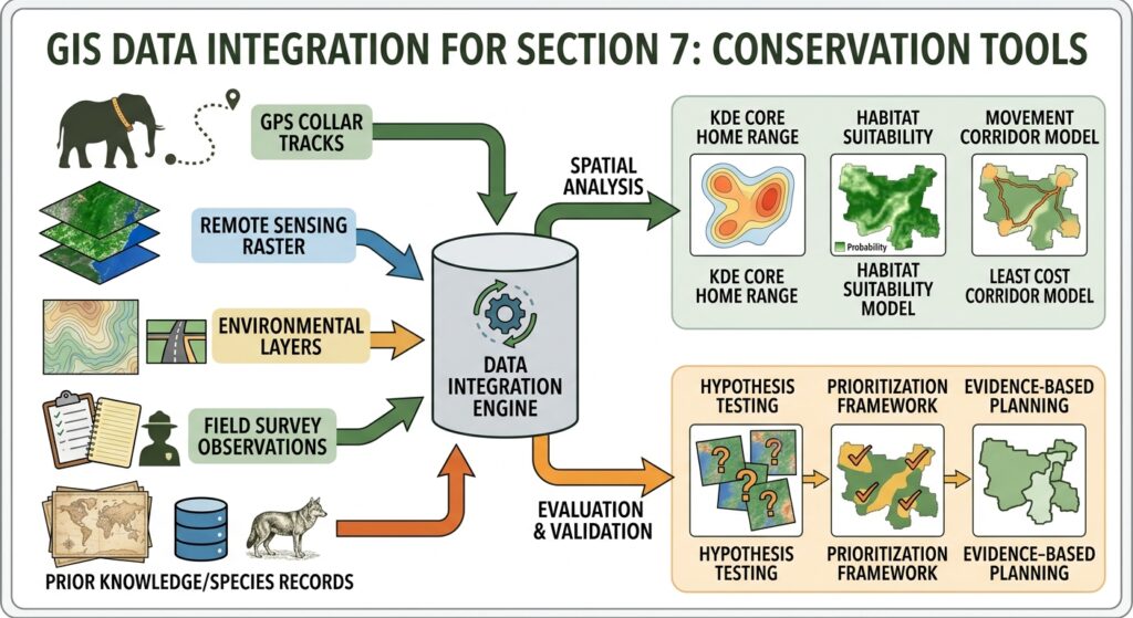
Conservation Goal	GIS Tool	Data Input Required
Estimate animal home range	MCP	GPS/telemetry points
Identify core-use areas	KDE	GPS/telemetry points
Map suitable habitat	MCE / weighted raster overlay	Land cover, terrain, vegetation, water, disturbance
Identify movement barriers	Raster analysis	Roads, settlements, fences, land cover
Map potential corridors	Least Cost Path	Resistance surface + habitat patches
Monitor vegetation	NDVI/raster analysis	Satellite imagery
Analyze habitat fragmentation	Landscape metrics	Land-cover/land-use raster
Identify protected-area gaps	Overlay/intersection	Protected areas + habitat distribution
Analyze seasonal movement	Temporal/spatial analysis	GPS locations with timestamps
Validate predicted habitat	Spatial validation	Independent occurrence/tracking data

Conclusion

GIS provides conservation researchers with a powerful way to connect animal movement, habitat characteristics, and landscape structure. Mastering these three methods provides a strong foundation for using GIS in wildlife conservation analysis to support real-world protection strategies.

Three techniques form a useful foundation for wildlife conservation analysis:

MCP and KDE help describe where animals use the landscape.
MCE and raster overlays help model where suitable habitat may occur.
Least Cost Path analysis helps identify potential connections between fragmented habitats.

The most effective conservation workflows combine these techniques rather than treating them as isolated mapping exercises. A researcher might begin with GPS locations, estimate home ranges, develop a habitat suitability model, construct a resistance surface, and finally identify potential corridors connecting important habitat patches.

The key is to remember that GIS does not replace ecological knowledge or field validation. It provides a spatial framework for testing hypotheses, identifying patterns, prioritizing areas for investigation, and supporting evidence-based conservation planning.