Advanced Spatial Index Tuning in PostGIS: GiST vs. SP-GiST vs. BRIN Indexes for Million-Row Tables

Introduction

Spatial query performance can deteriorate dramatically when geographic datasets grow from thousands to millions of records. A query that once returned nearby infrastructure assets in milliseconds may eventually trigger expensive sequential scans, consume excessive memory and disk bandwidth, or execute millions of unnecessary geometry comparisons.

The problem is not always a lack of indexing. Database engineers may already have a spatial index but still experience poor performance because the index structure does not match the geometry distribution, the table’s physical organization, or the query’s selectivity.

PostGIS supports three important spatial indexing strategies: GiST, SP-GiST, and BRIN. Each uses a different method to narrow down the rows that need further spatial evaluation.

GiST is the versatile default for most spatial workloads. SP-GiST partitions the search space and can perform well for suitable spatial distributions. BRIN summarizes the geographic extent of physical table blocks, trading precision for a dramatically smaller index when rows are spatially clustered.

Choosing correctly requires more than comparing index creation times. This guide explains the access methods, provides SQL for a reproducible benchmark involving 10 million points, and demonstrates how to evaluate bounding-box searches, point-in-polygon queries, index size, and execution plans.

The core principle is simple: spatial index performance depends on both the index structure and the relationship between geographic values and physical table storage.

1. Understand How PostGIS Spatial Indexes Work

Mastering Advanced Spatial Index Tuning in PostGIS starts with understanding how the database engine separates coarse bounding-box filtering from precise geometry evaluations.

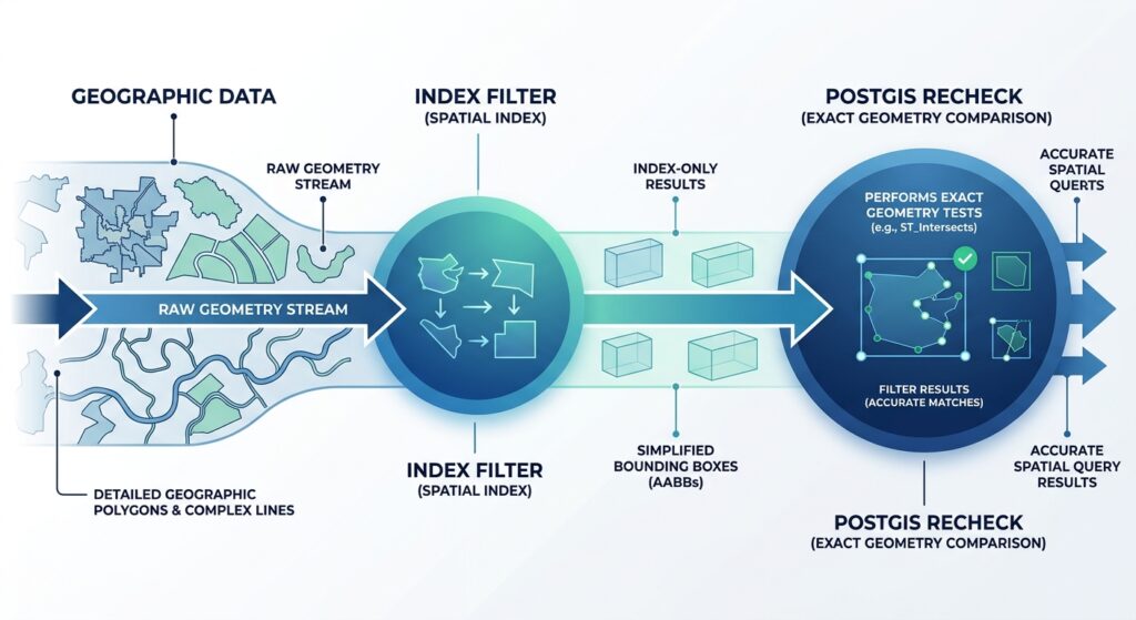
PostGIS spatial indexes generally store compact representations of geometry extents rather than every coordinate of each feature. For two-dimensional geometries, that representation is typically an axis-aligned bounding box.

The index identifies candidate rows, after which PostgreSQL or PostGIS evaluates the required spatial condition. This two-stage process is commonly called the primary and secondary filter.

For example:

SELECT id, geom
FROM infrastructure.assets
WHERE geom && ST_MakeEnvelope(
    350000, 9800000,
    370000, 9820000,
    3857
);

The && operator selects geometries whose bounding boxes overlap the requested envelope. It does not establish that arbitrary lines or polygons intersect the envelope exactly.

For an exact intersection query, use:

SELECT id
FROM infrastructure.assets
WHERE geom && ST_MakeEnvelope(
    350000, 9800000,
    370000, 9820000,
    3857
)
AND ST_Intersects(
    geom,
    ST_MakeEnvelope(
        350000, 9800000,
        370000, 9820000,
        3857
    )
);

The explicit bounding-box condition makes the candidate-selection stage visible, although many index-aware PostGIS predicates, including ST_Intersects, already incorporate an indexable bounding-box filter.

This behavior is important when benchmarking. An index can eliminate most irrelevant rows but still incur substantial exact-geometry computation if its candidate set contains many false positives.

See the official PostGIS spatial index documentation for the details of index-aware operators and access methods.

2. GiST: The General-Purpose Spatial Index

GiST, or Generalized Search Tree, is the standard starting point for PostGIS spatial indexing. PostGIS implements an R-tree-style spatial index on top of GiST, making it suitable for a broad range of geographic workloads. When evaluating spatial partition structures, incorporating Advanced Spatial Index Tuning in PostGIS principles ensures that point-heavy distributions select the right quadtree or kd-tree access method without sacrificing query flexibility.

How GiST works

GiST organizes geometry bounding boxes into a hierarchical search structure. A query first traverses index entries whose extents may satisfy the requested spatial condition, then visits the relevant table rows.

This approach is particularly effective when geographic queries are selective and the index can eliminate most of the table.

Typical workloads include:

• Finding points within a radius or rectangular extent.
• Intersecting road networks with administrative boundaries.
• Testing whether facilities fall inside service areas.
• Performing spatial joins between points, lines, and polygons.
• Supporting interactive web-map queries against changing datasets.

Create and inspect a GiST index

CREATE INDEX assets_geom_gix
ON infrastructure.assets
USING GIST (geom);

ANALYZE infrastructure.assets;

For a large production table, CREATE INDEX CONCURRENTLY can reduce disruption to concurrent writes, at the cost of additional work and operational complexity.

The default geometry index is two-dimensional. If the application needs indexed searches across multiple dimensions, investigate the appropriate n-dimensional operator class rather than assuming a conventional 2D index will accelerate every 3D predicate.

GiST tuning considerations

Bounding-box overlap: Long diagonal lines, extensive polygons, and dispersed multipart geometries can have bounding boxes that cover substantial irrelevant space. This increases the number of candidates and exact rechecks.

Index size: GiST indexes can become substantial on large, complex datasets. Their storage footprint and maintenance overhead must be considered alongside query latency.

Write workload: Inserts, updates, and deletes maintain index structures. A workload with frequent geometry changes may need different tuning from a read-mostly analytical table.

Physical locality: Clustering heap rows around a spatial ordering can sometimes improve locality for range queries, although the benefit depends on the workload and maintenance requirements.

GiST is usually the first index to benchmark because it offers the broadest baseline for conventional PostGIS applications. See the PostGIS GiST index reference.

3. SP-GiST: Partitioning the Search Space

SP-GiST stands for Space-Partitioned Generalized Search Tree. Instead of organizing entries primarily through overlapping bounding-box hierarchies, it supports partitioned structures such as quadtrees and kd-trees.

These structures repeatedly divide a search space into regions. The regions do not have to contain equal numbers of records, making the method suitable for distributions that align well with the chosen partitioning strategy.

When SP-GiST makes sense

SP-GiST is worth testing for point-heavy datasets, spatial distributions with useful partition boundaries, and workloads dominated by supported spatial operators.

For example, a database of millions of monitoring stations, customer locations, or sampled coordinates may be a good candidate for a direct GiST-versus-SP-GiST comparison.

However, SP-GiST should not be assumed to outperform GiST for every point dataset. Concentrated urban clusters, irregular distributions, complex geometries, and different query selectivities can change the outcome.

Create an SP-GiST index

For a standard two-dimensional PostGIS geometry column:

CREATE INDEX assets_geom_spgist
ON infrastructure.assets
USING SPGIST (geom);

ANALYZE infrastructure.assets;

The default operator class is two-dimensional. PostGIS also provides a 3D operator class for suitable workloads:

CREATE INDEX assets_geom_spgist_3d
ON infrastructure.assets
USING SPGIST (geom spgist_geometry_ops_3d);

Only choose the 3D variant after confirming that the application’s queries use the corresponding indexed operators.

Important limitations

SP-GiST is not a universal replacement for GiST. PostGIS documents its supported spatial operators, and the applicable operator class determines which conditions can use the index. In particular, PostGIS documents that its SP-GiST geometry index does not currently support the same k-nearest-neighbor search capability commonly used with GiST.

For applications that depend on distance-ordered searches such as:

SELECT id, geom
FROM infrastructure.assets
ORDER BY geom <-> ST_SetSRID(
    ST_MakePoint(360000, 9810000),
    3857
)
LIMIT 20;

verify that the selected index and operator combination supports the intended plan. Do not assume that any spatial index will automatically accelerate every distance operation.

The official PostGIS SP-GiST documentation lists the supported operators and relevant index definitions.

4. BRIN: Compact Indexing for Spatially Ordered Tables

BRIN, or Block Range Index, takes a substantially different approach. Instead of storing a detailed spatial search hierarchy, it summarizes the geographic extent of groups of consecutive heap pages.

When a query arrives, PostgreSQL evaluates these summaries to identify physical page ranges that may contain matching geometries. It then reads the relevant heap pages and checks individual rows.

Why BRIN can be dramatically smaller

A typical BRIN spatial index stores a summary for each block range rather than a separate detailed index entry for every feature.

The default spatial pages_per_range setting is 128. Increasing this value reduces the number of summaries and generally shrinks the index, but it can also increase the number of heap pages that need to be examined. Decreasing it creates finer summaries at the cost of a larger index.

For very large tables, the trade-off can be attractive: the index consumes little storage and can be quick to build.

However, BRIN’s effectiveness depends strongly on physical spatial locality.

If neighboring table pages contain geographically nearby points, each page-range summary may cover a small area. If consecutive rows contain randomly scattered global coordinates, each summary may span much of the world, making it less useful for selective geographic queries.

Create and tune a BRIN index

CREATE INDEX assets_geom_brin
ON infrastructure.assets
USING BRIN (geom)
WITH (pages_per_range = 32);

ANALYZE infrastructure.assets;

The value 32 is an experiment, not a universal optimum. Compare it with the default and several alternative values using the actual query distribution.

BRIN is especially worth evaluating for large, append-oriented or read-mostly spatial datasets whose rows are physically ordered by geography. Examples include spatially clustered observation archives and large point collections loaded in a geographic sort order.

PostGIS also documents BRIN support for geometry and geography, as well as higher-dimensional operator classes. Its supported spatial operations are more limited than a general-purpose GiST index.

Maintain BRIN summaries

Unlike GiST and SP-GiST, BRIN summaries are not maintained in the same way for every newly inserted value. New page ranges may require summarization, and unsummarized or poorly summarized ranges can reduce the effectiveness of the index.

After applicable data changes, inspect summary coverage and consider:

SELECT brin_summarize_new_values(
    'infrastructure.assets_geom_brin'::regclass
);

Routine maintenance and PostgreSQL’s BRIN summarization settings should be incorporated into the ingestion workflow.

See PostGIS BRIN index documentation for spatial ordering, summary behavior, and page-range tuning. For large, spatially sorted tables, applying Advanced Spatial Index Tuning in PostGIS with Block Range Indexes minimizes disk footprints while maintaining rapid range query responses on append-heavy workloads.

5. Benchmark All Three Indexes on 10 Million Rows

A meaningful PostGIS index comparison must control for dataset size, spatial distribution, physical row ordering, query selectivity, and cache state. The following workflow creates a 10-million-point test table and uses the same physically ordered relation to compare the three access methods.

Run the test on a staging database with enough disk space and time for table construction and index creation. These are benchmark instructions, not measured performance results.

Step 1: Generate the benchmark table

CREATE UNLOGGED TABLE bench_points AS
SELECT
    i AS id,
    ST_SetSRID(
        ST_MakePoint(
            random() * 1000000,
            random() * 1000000
        ),
        3857
    ) AS geom
FROM generate_series(1, 10000000) AS s(i)
ORDER BY geom;

ANALYZE bench_points;

This creates ten million synthetic points within a 1,000,000-by-1,000,000-unit square in EPSG:3857 and sorts them spatially using the geometry ordering supported by the installed PostGIS version.

The table is UNLOGGED to reduce test setup WAL overhead; it is not appropriate for durable production data. The benchmark uses synthetic, uniformly distributed points, so the results should not be extrapolated directly to complex polygon or road-network datasets.

Step 2: Benchmark the bounding-box query

Use the same spatial extent for every index trial:

EXPLAIN (ANALYZE, BUFFERS)
SELECT count(*)
FROM bench_points
WHERE geom && ST_MakeEnvelope(
    400000, 400000,
    600000, 600000,
    3857
);

Create one index at a time, run ANALYZE, capture the plan and timings, then drop that index before testing the next method.

GiST trial:

CREATE INDEX bench_points_gist
ON bench_points USING GIST (geom);

ANALYZE bench_points;

SP-GiST trial:

DROP INDEX bench_points_gist;

CREATE INDEX bench_points_spgist
ON bench_points USING SPGIST (geom);

ANALYZE bench_points;

BRIN trial:

DROP INDEX bench_points_spgist;

CREATE INDEX bench_points_brin
ON bench_points USING BRIN (geom)
WITH (pages_per_range = 32);

ANALYZE bench_points;

Execute the query after each index is built. Record index creation time separately from query execution time.

Because the test table is spatially ordered, it represents a favorable starting condition for BRIN. For contrast, create a second table in a non-spatial order and repeat the BRIN test. This reveals how much the method depends on physical clustering.

Step 3: Benchmark point-in-polygon filtering

Bounding-box queries measure candidate selection but do not fully represent topological filtering. Add an exact spatial predicate:

EXPLAIN (ANALYZE, BUFFERS)
SELECT count(*)
FROM bench_points
WHERE ST_Contains(
    ST_MakeEnvelope(
        400000, 400000,
        600000, 600000,
        3857
    ),
    geom
);

For point geometries, the rectangular containment test is straightforward, although the query still needs to identify points in the target area. With complex polygons, bounding-box false positives and exact geometry complexity can materially alter the cost.

Benchmark a representative polygon from your actual dataset as a second test rather than treating this rectangle as representative of all point-in-polygon workloads.

Step 4: Measure index size

After each trial, capture the index’s disk footprint:

SELECT
    indexrelid::regclass AS index_name,
    pg_size_pretty(
        pg_relation_size(indexrelid)
    ) AS index_size
FROM pg_index
WHERE indrelid = 'bench_points'::regclass;

For index-creation time, use \timing on in psql or collect timing in the test harness. Repeat query measurements several times, allow comparable cache warm-up, and compare medians rather than relying on a single execution.

Step 5: Interpret the execution plan

Look for the following plan nodes and indicators:

• Index Scan / Bitmap Index Scan: Indicates index-assisted retrieval. A sequential scan may still be correct for broad queries that return a large proportion of the table.
• Rows Removed by Index Recheck: Signals candidate rows that failed a subsequent condition.
• Buffers: shared hit/read: Helps distinguish repeated access to cached pages from physical reads.
• Actual rows versus estimated rows: Highlights possible planner estimation problems.
• Execution Time: Compare alongside row counts and buffer activity; time alone does not explain why one plan wins.

The PostgreSQL EXPLAIN guide explains execution plans, buffer reporting, and the caveats around interpreting benchmark results.

6. Compare Query Performance and Storage Overhead

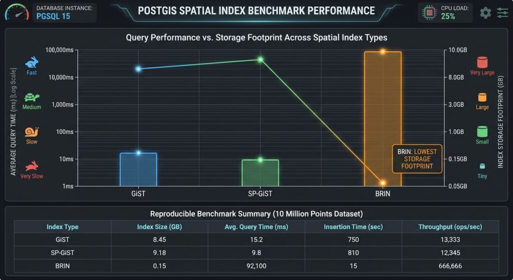
Populate the chart with the measured results from the preceding benchmark. Do not use invented universal latency or storage figures: hardware, PostGIS and PostgreSQL versions, geometry types, table layout, and selectivity materially affect the outcome.

The expected qualitative trade-offs are:

Criterion	GiST	SP-GiST	BRIN
Selective spatial queries	Strong general-purpose baseline	Can be competitive for suitable distributions	Depends heavily on spatial locality
Complex geometry support	Broad	Operator-class dependent	Limited compared with GiST
Index storage	Often moderate to large	Workload dependent	Usually very small
Index construction	Can be relatively expensive	Must be measured	Usually fast
Update-heavy workloads	General-purpose choice	Workload dependent	Requires careful summarization and maintenance
Physical row ordering	Can benefit from locality	Can benefit from locality	Critical to effectiveness
Best initial use case	Most general spatial datasets	Alternative for supported partition-friendly workloads	Large, spatially clustered tables

These are architectural expectations rather than benchmark rankings. In particular, BRIN may perform acceptably when a query returns many records, while a very selective query on poorly clustered data can force it to inspect too much of the heap.

7. Advanced Spatial Index Tuning in PostGIS: Beyond the Index Type

Changing the index access method is only one part of tuning. Before replacing a working GiST index, examine the query and table design.

Keep spatial predicates index-aware. Avoid transforming the indexed geometry column inside every filter when a constant query geometry can instead be transformed once into the column’s CRS. Ensure the compared geometries have compatible SRIDs.

Refresh statistics. Use ANALYZE after bulk loads and significant changes to the dataset. Poor cardinality estimates can cause the planner to choose a sequential scan or an inefficient join strategy.

Separate mixed workloads. A table containing millions of points alongside large, irregular multipolygons may behave differently from a point-only table. Partitioning by a meaningful attribute, geometry type, region, or time period can make indexing and maintenance more predictable.

Review rechecks and candidate ratios. An index returning thousands of candidates for a query that matches only a few dozen rows may be structurally or distributionally inefficient. Geometry subdivision, more selective predicates, or an alternative index may help, depending on the dataset.

Measure write costs. More indexes increase storage consumption and the work required to maintain indexed data. Avoid adding multiple competing spatial indexes to the same production table without demonstrating that they improve the workload.

Test with representative concurrency. A single-user microbenchmark does not capture buffer contention, concurrent updates, connection pressure, or the I/O behavior of a busy spatial API.

8. SEO Interlinking and Related Technical Guides

Link this article to adjacent tutorials that address spatial query patterns, alternative indexing schemes, and data architecture.

• PostGIS Spatial Window Functions: Link from the query tuning section to a guide on spatial ranking, neighborhood aggregation, and analytical functions. Suggested slug: /postgis-spatial-window-functions/
• H3 vs. Geohash Indexing: Link from the BRIN spatial-ordering discussion to a comparison of spatial cell IDs for partitioning, aggregation, and coarse geographic filtering. Suggested slug: /h3-vs-geohash-spatial-indexing/
• Spatial Data Lakehouse Architecture: Link from the million-row benchmark section to an article about separating transactional spatial workloads from large-scale analytical processing. Suggested slug: /spatial-data-lakehouse-architecture/

These are suggested internal URLs, not verified live pages. Replace them with the actual published URLs before publication.

Conclusion

The right PostGIS spatial index is the one that matches the geometry distribution, query operators, and physical organization of the workload.

GiST provides the strongest general starting point for spatial range searches, topological filtering, and mixed geometry types. SP-GiST offers an alternative partition-based structure that deserves measurement where its operator support and data distribution are a good fit. BRIN can dramatically reduce indexing storage and creation costs for large, geographically clustered tables, but loses much of its advantage when neighboring heap pages contain globally scattered geometries.

For million-row and ten-million-row workloads, benchmark index size, index-build time, execution time, buffer activity, and exact-filter cost together. Validate the results on representative queries and repeat the tests under realistic cache and concurrency conditions.

The practical optimization sequence is to verify index-aware SQL, refresh statistics, establish a GiST baseline, test SP-GiST where appropriate, and evaluate BRIN when physical spatial ordering can be maintained.

That disciplined approach turns PostGIS Spatial Index Tuning GiST SP-GiST BRIN from a theoretical index comparison into a measurable database engineering decision.

Ready to eliminate database bottlenecks and scale your spatial infrastructure? Reach out for expert guidance and professional project support to master Advanced Spatial Index Tuning in PostGIS today, and transform your million-row workflows into lightning-fast spatial applications!