
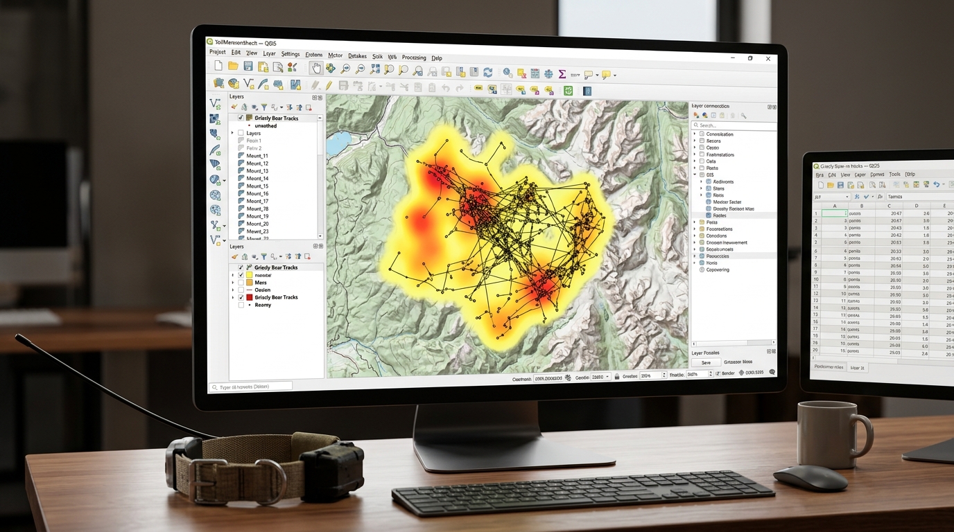
Integrating GPS Telemetry Data with Open-Source GIS for Wildlife Tracking and Home Range Analysis
Modern wildlife conservation and spatial ecology rely heavily on high-resolution GPS satellite telemetry. Traditional VHF radio-tracking methods—while foundational—have largely been superseded by collars equipped with GPS, Iridium, Argos, or cellular data transmission. These advanced devices log thousands of precise coordinate locations per animal over multi-year deployments, providing unprecedented insight into animal movement, habitat selection, migration corridors, and human-wildlife conflict zones.
However, raw telemetry feeds generated by collar hardware are rarely ready for immediate ecological analysis. They arrive as massive tabular CSV files laden with spatial noise, temporal irregularities, and duplicate coordinate fixes. Processing this data requires a robust geospatial workflow capable of cleaning telemetry streams, constructing movement trajectories, and calculating home range estimators.
In this applied guide, we explore a production-grade workflow using open-source GIS tools (QGIS, Python, and GeoPandas) to transform raw GPS tracking data into actionable home range models and utilization distributions.
The Role of Telemetry and Spatial Ecology in Conservation
Understanding how wildlife utilizes geographic space is critical for designing effective protected areas and wildlife corridors. The concept of a home range—defined by Burt (1943) as the area traversed by an individual in its normal activities of food gathering, mating, and caring for young—serves as the primary spatial unit in terrestrial ecology.
When conducting animal movement analysis in QGIS, researchers transition from simple static point plotting to dynamic spatial modeling. By combining open-source GIS utilities with scripting languages like Python and R, conservation scientists can automate ingestion pipelines, filter GPS error anomalies, and compute standard home range metrics such as Minimum Convex Polygons (MCP) and Kernel Density Estimation (KDE).
Step 1: Importing Raw CSV Telemetry Data and Constructing Trajectory Lines
GPS collars typically export time-series logs containing device IDs, timestamps, latitudes, longitudes, elevation values, and dilution of precision (DOP) metrics. Our first objective is to import these tabular records into a spatial environment and reconstruct continuous movement trajectories.
Importing GPS Telemetry Data in QGIS
-
Open QGIS and navigate to Layer > Add Layer > Add Delimited Text Layer.
-
Select your CSV file containing telemetry logs.
-
Define the X field as
longitudeand the Y field aslatitude. -
Set the Coordinate Reference System (CRS) to geographic WGS 84 (
EPSG:4326). -
Click Add to load the point layer into the map canvas.
Constructing Trajectory Lines in Python
To analyze movement between consecutive fixes, point features must be sorted chronologically by timestamp and converted into ordered
LineString vector trajectories. We accomplish this using Python and geopandas:Python
import pandas as pd
import geopandas as geospatial
from shapely.geometry import LineString, Point

# Load raw telemetry CSV
df = pd.read_csv("wildlife_telemetry_raw.csv")

# Convert timestamp column to datetime and sort chronologically per animal ID
df['timestamp'] = pd.to_datetime(df['timestamp'])
df = df.sort_values(by=['animal_id', 'timestamp'])

# Convert DataFrame to GeoDataFrame in WGS84
gdf_points = geospatial.GeoDataFrame(
    df, geometry=geospatial.points_from_xy(df['longitude'], df['latitude']), crs="EPSG:4326"
)

# Re-project to local metric CRS (e.g., UTM Zone 37S - EPSG:32737) for accurate distance calculations
gdf_projected = gdf_points.to_crs("EPSG:32737")

# Group points by individual animal to build trajectory linestrings
trajectories = []
for animal_id, group in gdf_projected.groupby('animal_id'):
    if len(group) > 1:
        coords = [Point(geom.x, geom.y) for geom in group.geometry]
        line = LineString(coords)
        trajectories.append({
            'animal_id': animal_id,
            'fix_count': len(group),
            'geometry': line
        })

gdf_trajectories = geospatial.GeoDataFrame(trajectories, crs="EPSG:32737")
print(f"Constructed movement trajectories for {len(gdf_trajectories)} individual animals.")
Step 2: Cleaning Outlier GPS Points (Speed and Fix-Rate Filters)
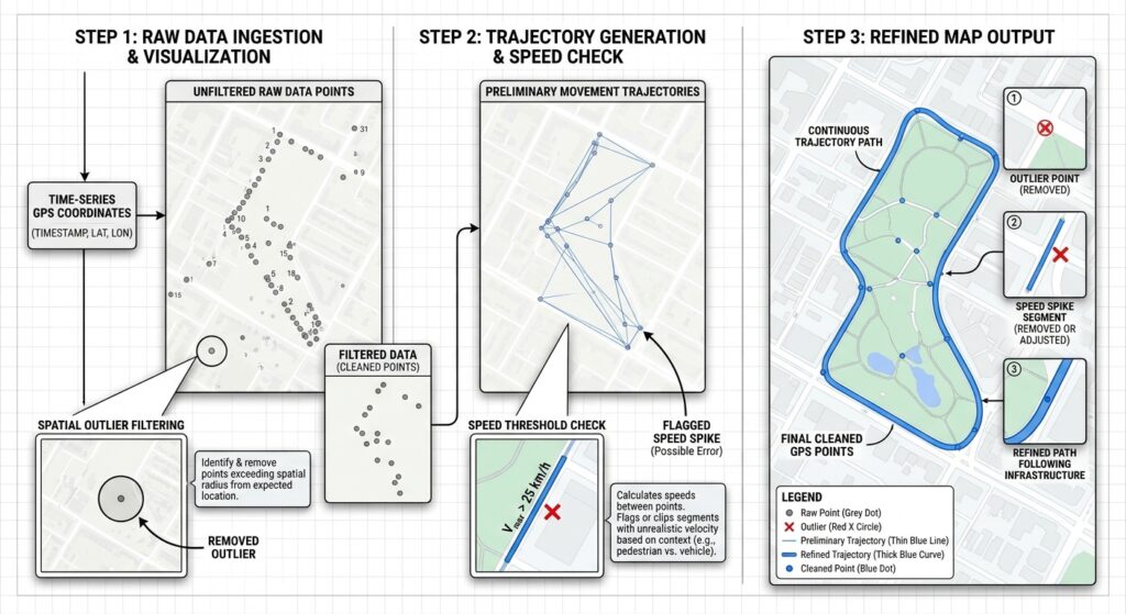
Raw GPS fixes inevitably contain erroneous locations caused by atmospheric interference, satellite geometry degradation, or physical obstruction (e.g., dense forest canopies or steep gorges). These errors manifest as unrealistic spatial jumps, where an animal appears to teleport across impossible distances between consecutive pings.
Implementing Speed and PDOP Filters
We clean the dataset by enforcing two primary validation criteria:
-
Geometric Dilution of Precision (PDOP): Removing fixes where satellite configuration geometry yields high positional uncertainty (typically PDOP > 5.0).
-
Physiological Speed Thresholds: Calculating instantaneous movement speed between consecutive fixes based on elapsed time and distance. If the required speed exceeds the maximum biological movement capacity of the species (e.g., > 30 km/h for large ungulates), the point is flagged as an outlier.
Python
import numpy as np

def clean_telemetry_data(group_df, max_speed_kmh=25.0, max_pdop=5.0):
    """
    Filters GPS telemetry points based on PDOP and biologically impossible movement speeds.
    """
    # Filter by PDOP if present in columns
    if 'pdop' in group_df.columns:
        group_df = group_df[group_df['pdop'] <= max_pdop]

    group_df = group_df.sort_values('timestamp').reset_index(drop=True)
    valid_indices = [0]  # Keep first fix

    for i in range(1, len(group_df)):
        p1 = group_df.loc[i-1, 'geometry']
        p2 = group_df.loc[i, 'geometry']
        t1 = group_df.loc[i-1, 'timestamp']
        t2 = group_df.loc[i, 'timestamp']

        # Distance in meters
        dist_m = p1.distance(p2)
        # Time difference in hours
        time_diff_hrs = (t2 - t1).total_seconds() / 3600.0

        if time_diff_hrs > 0:
            speed_kmh = (dist_m / 1000.0) / time_diff_hrs
            if speed_kmh <= max_speed_kmh:
                valid_indices.append(i)
        else:
            # Duplicate timestamps
            continue

    return group_df.loc[valid_indices]

# Apply cleaning filter per animal
cleaned_dfs = []
for animal_id, group in gdf_projected.groupby('animal_id'):
    cleaned_group = clean_telemetry_data(group)
    cleaned_dfs.append(cleaned_group)

gdf_cleaned = geospatial.concat(cleaned_dfs, ignore_index=True)
print(f"Retained {len(gdf_cleaned)} valid telemetry fixes out of {len(gdf_points)} total raw points.")
Step 3: Computing Minimum Convex Polygons (MCP) for Core Habitat Estimation
The Minimum Convex Polygon (MCP) is the oldest and most widely cited home range estimator in wildlife ecology. It constructs the smallest convex boundary that encloses all observed telemetry locations for an individual animal.
Executing MCP in QGIS
-
Open the Processing Toolbox in QGIS (
Ctrl + Alt + T). -
Search for and select the Minimum bounding geometry tool under the Vector geometry group.
-
Set your cleaned GPS point layer as the Input layer.
-
Set the Geometry type to
Convex Hull. -
Under Field, select your
animal_idattribute to generate individual MCP boundaries per animal. -
Run the tool.
Limitations of MCP
While MCP provides a standardized macro-scale metric for comparing range sizes across different species or management zones, it suffers from significant ecological drawbacks:
-
Inclusion of Unused Habitat: Because it connects outermost perimeter points, MCP often encompasses large swaths of terrain (such as deep water bodies or impassable cliffs) that the animal never actually visited.
-
Sample Size Sensitivity: MCP area scales monotonically with sample size. As collar deployment duration increases and more fixes are recorded, the polygon continuously expands to capture outlier exploratory movements.
Step 4: Generating Probabilistic Home Ranges Using Kernel Density Estimation (KDE) and Utilization Distributions
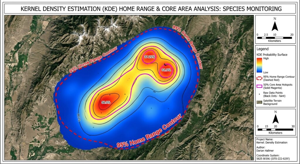
To overcome the geometric limitations of MCP, spatial ecologists rely on probabilistic home range estimators known as Utilization Distributions (UD). The most prevalent technique is Kernel Density Estimation (KDE), which calculates a continuous probability surface representing the relative frequency with which an animal occurs across space.
The Mechanics of KDE
KDE places a bivariate probability density function (kernel)—typically a 2D Gaussian bell curve—over each GPS fix location. The individual kernels are summed across a regular spatial grid and normalized to form a continuous surface where the volume under the surface integrates to 1.
-
95% Home Range Contour: Represents the outer boundary enclosing 95% of the animal’s utilization probability volume, capturing its general home range.
-
50% Core Area Contour: Encloses the inner 50% probability volume, highlighting core resting, foraging, or breeding hotspots.
Selecting the Bandwidth Parameter ($h$)
The smoothness of a KDE surface is governed by the smoothing parameter, or bandwidth ($h$). Selecting an inappropriate bandwidth severely distorts home range estimates:
-
Undersmoothing: Creates fragmented, isolated islands around individual GPS points.
-
Oversmoothing: Flattens the probability surface into a generalized blob that obscures localized habitat utilization.
Advanced practitioners utilize Reference Bandwidth ($h_{ref}$) or Least Squares Cross-Validation (LSCV) to determine optimal smoothing parameters.
Executing KDE in Python via SciPy
Using our cleaned metric GeoDataFrame, we can compute 2D Kernel Density Estimation surfaces and export the resulting probabilistic grid into georeferenced raster layers, leveraging efficient raster optimization strategies:
Python
from scipy.stats import gaussian_kde
import rasterio
from rasterio.transform import from_origin

def generate_kde_raster(animal_subset_gdf, output_filename, cell_size=30.0, bandwidth_factor=1.2):
    """
    Computes 2D Gaussian KDE for an individual animal and exports to GeoTIFF.
    """
    coords = np.array([[geom.x, geom.y] for geom in animal_subset_gdf.geometry])
    x = coords[:, 0]
    y = coords[:, 1]

    # Initialize Gaussian KDE
    kde = gaussian_kde(coords.T)

    # Apply bandwidth adjustment factor
    kde.set_bandwidth(kde.factor * bandwidth_factor)

    # Define bounding grid with cell_size resolution (e.g., 30m pixels)
    buffer = 1000.0  # 1km buffer around points
    xmin, ymin, xmax, ymax = x.min() - buffer, y.min() - buffer, x.max() + buffer, y.max() + buffer

    x_grid = np.arange(xmin, xmax, cell_size)
    y_grid = np.arange(ymin, ymax, cell_size)
    xx, yy = np.meshgrid(x_grid, y_grid)
    grid_coords = np.vstack([xx.ravel(), yy.ravel()])

    # Evaluate density across grid
    z = kde(grid_coords).reshape(xx.shape)

    # Normalize density values so integral equals 1
    z_sum = np.sum(z) * (cell_size ** 2)
    z_normalized = z / z_sum

    # Export to GeoTIFF using Rasterio
    transform = from_origin(xmin, ymax, cell_size, cell_size)
    raster_data = z_normalized.astype(np.float32)

    with rasterio.open(
        output_filename,
        'w',
        driver='GTiff',
        height=raster_data.shape[0],
        width=raster_data.shape[1],
        count=1,
        dtype=raster_data.dtype,
        crs="EPSG:32737",
        transform=transform,
    ) as dst:
        dst.write(raster_data, 1)

    print(f"Exported Utilization Distribution raster to {output_filename}")

# Run KDE generation for a specific animal
sample_animal = gdf_cleaned[gdf_cleaned['animal_id'] == 'ELEPHANT_042']
generate_kde_raster(sample_animal, "elephant_042_ud.tif")
For advanced multi-individual habitat analyses, these continuous utilization rasters can be paired with vector point layers to evaluate resource selection functions (RSF) or integrated directly into broader spatial point pattern analysis workflows to test for spatial clustering against environmental covariates.
Summary
Integrating GPS telemetry data with open-source GIS tools provides conservation scientists and wildlife managers with a powerful, flexible framework for monitoring animal movement and spatial ecology. By moving from raw tabular CSV logs to cleaned metric trajectories, filtering GPS outlier errors, computing traditional Minimum Convex Polygons, and generating probabilistic Kernel Density Estimation utilization distributions, researchers can accurately map core habitats, identify critical migration bottlenecks, and formulate data-driven wildlife conservation strategies.