
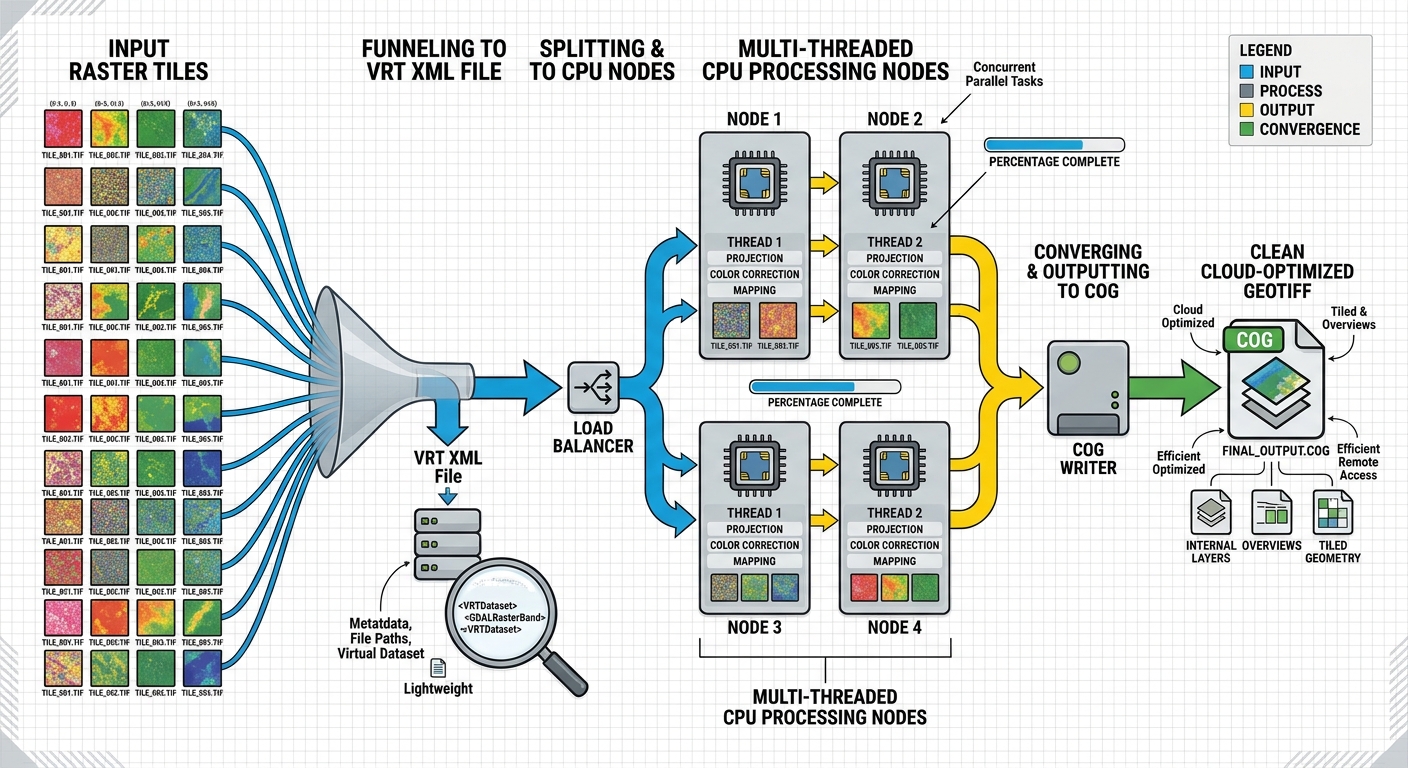
Optimizing Raster Processing Performance with GDAL Multi-Threading and VRT (Virtual Raster) Files
Processing a handful of GeoTIFF files is rarely a performance problem. The situation changes dramatically when a workflow involves hundreds of multi-gigabyte satellite scenes, DEM tiles, orthophotos, or other raster datasets.
A conventional raster workflow may repeatedly read source tiles, create intermediate files, write temporary mosaics to disk, and then read those intermediates again for reprojection, clipping, resampling, or conversion. The result is often a pipeline constrained less by CPU performance than by disk I/O, memory consumption, temporary storage, and unnecessary data duplication.
GDAL provides two particularly powerful mechanisms for addressing these bottlenecks: multi-threaded processing and Virtual Raster Tables (VRTs).
A VRT allows GDAL to describe a mosaic or raster transformation using a lightweight XML file rather than immediately creating another physical raster. Multi-threading can then accelerate computationally expensive operations such as reprojection and resampling.
Together, these techniques provide an efficient architecture for large raster pipelines:
Hundreds of source GeoTIFFs
          │
          ▼
     gdalbuildvrt
          │
          ▼
      mosaic.vrt
          │
     ┌────┴────┐
     │         │
     ▼         ▼
   Clip     Reproject
     │         │
     └────┬────┘
          ▼
     gdalwarp
  multi-threaded
          │
          ▼
   Optimized GeoTIFF
          │
          ▼
         COG
This guide explains how to build that workflow and how to benchmark it properly.
1. Why Large Raster Workflows Become Slow
Raster processing involves several different resources, and optimizing one does not automatically optimize the others.
1.1 Disk I/O
A raster pipeline can become I/O-bound when it repeatedly performs operations such as:
- Read hundreds of source files.
- Write an intermediate mosaic.
- Read the mosaic again.
- Write a clipped raster.
- Read the clipped raster.
- Reproject it.
- Write another intermediate.
- Compress the final result.
If the original dataset contains hundreds of gigabytes, every unnecessary read and write can become expensive.
For example:
Tiles → Physical Mosaic → Clip → Reproject → Compressed Outputmay require several complete passes over the data.
A VRT changes the architecture:
Tiles → VRT → Reproject/Clip → Final OutputThe VRT does not normally contain the complete raster pixel data. Instead, it describes how the source datasets should be accessed.
1.2 Memory Pressure
It is tempting to assume that faster raster processing simply requires loading more data into RAM.
That is rarely practical with multi-gigabyte datasets.
A 10,000 × 10,000 raster containing Float32 values requires approximately:
10,000 × 10,000 × 4 bytes
= 400,000,000 bytes
≈ 381 MiB
before accounting for additional bands, buffers, intermediate arrays, GDAL caches, and processing overhead.
A large mosaic can therefore exceed available RAM very quickly.
GDAL’s block-based architecture allows applications to process raster regions without loading the entire dataset into memory.
2. What Is a GDAL Virtual Raster (VRT)?
A GDAL Virtual Raster (VRT) is an XML-based raster description that references one or more underlying raster datasets.
Instead of physically copying pixels into a new mosaic, a VRT stores information such as:
- source filenames
- raster dimensions
- geotransforms
- coordinate systems
- bands
- pixel offsets
- source windows
- nodata values
- resampling information
- masks
- overviews
- data types
A simplified VRT concept looks like this:
<VRTDataset rasterXSize="10000" rasterYSize="10000">

  <SRS>...</SRS>

  <VRTRasterBand dataType="Float32" band="1">

    <SimpleSource>
      <SourceFilename>tile_001.tif</SourceFilename>
      <SourceBand>1</SourceBand>
    </SimpleSource>

    <SimpleSource>
      <SourceFilename>tile_002.tif</SourceFilename>
      <SourceBand>1</SourceBand>
    </SimpleSource>

  </VRTRasterBand>

</VRTDataset>
The important point is that tile_001.tif and tile_002.tif remain the original datasets.
The VRT acts as a virtual representation of the combined raster.
VRT is not a compressed raster
A VRT normally does not make the underlying pixels smaller.
Instead, it reduces unnecessary data movement and allows GDAL to construct a logical raster view without immediately writing a new physical raster.
This makes VRTs particularly useful for:
- mosaicking
- clipping
- raster subsetting
- temporary processing stages
- reprojection pipelines
- large raster collections
- experimentation
- automated ETL pipelines
3. Build a Virtual Raster Mosaic with gdalbuildvrt
Suppose a directory contains:
dem/
├── tile_001.tif
├── tile_002.tif
├── tile_003.tif
├── ...
└── tile_500.tif
Instead of immediately merging those files into one enormous GeoTIFF, create a VRT.
gdalbuildvrt dem_mosaic.vrt dem/*.tifGDAL creates:
dem_mosaic.vrtThe source TIFFs remain unchanged.
The resulting architecture is:
tile_001.tif ─┐
tile_002.tif ─┤
tile_003.tif ─┤
     ...      ├──► dem_mosaic.vrt
tile_500.tif ─┘
This operation can be dramatically cheaper than physically mosaicking the files because GDAL is primarily constructing metadata describing the mosaic.
Use a tile index for very large collections
For extremely large datasets, explicitly supplying hundreds or thousands of filenames can become inconvenient.
A file list can be used:
find /data/dem -name "*.tif" > dem_tiles.txtThen:
gdalbuildvrt dem_mosaic.vrt -input_file_list dem_tiles.txtThis is useful in automated pipelines where the list of available scenes changes over time.
Check the VRT
Use:
gdalinfo dem_mosaic.vrtYou can inspect:
- raster dimensions
- coordinate reference system
- number of bands
- pixel size
- extent
- nodata information
- metadata
A VRT therefore becomes a convenient intermediate dataset for subsequent GDAL operations.
4. Why VRTs Reduce Redundant Disk Writing
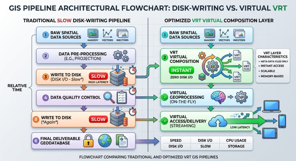
Consider a traditional workflow:
500 TIFFs
   ↓
Write 300 GB mosaic.tif
   ↓
Read 300 GB mosaic.tif
   ↓
Write clipped.tif
   ↓
Read clipped.tif
   ↓
Write reprojected.tif
The physical mosaic may be temporary and only exist to support another operation.
With VRT:
500 TIFFs
   ↓
Create tiny VRT descriptor
   ↓
Read required source blocks
   ↓
Warp / resample / clip
   ↓
Write final output
The key optimization is not that VRT makes the actual computation disappear.
Instead, it eliminates an unnecessary physical intermediate dataset.
That distinction is important when designing production pipelines.
5. How GDAL Multi-Threading Speeds Up Processing
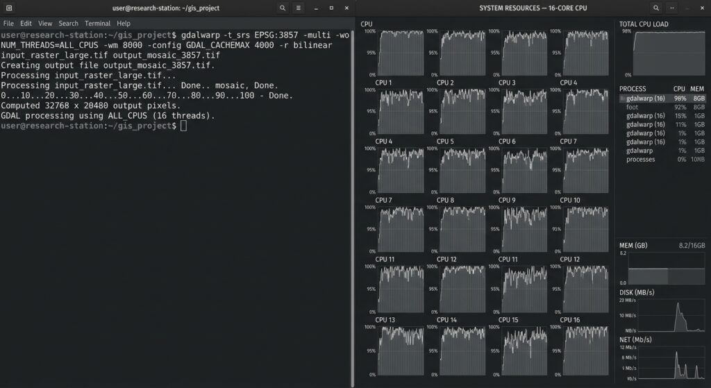
VRTs primarily address data organization and I/O. Multi-threading addresses CPU-intensive operations.
A raster operation such as reprojection may involve:
Source pixel
      ↓
Coordinate transformation
      ↓
Resampling
      ↓
Nodata handling
      ↓
Output block
For large rasters, these calculations can consume substantial CPU time.
GDAL’s warping machinery supports multi-threaded processing.
A common pattern is:
gdalwarp \
  -multi \
  -wo NUM_THREADS=ALL_CPUS \
  input.vrt \
  output.tif
Two concepts are important here.
-multi
For gdalwarp, -multi enables multi-threaded I/O/processing behavior so reading and writing can overlap with computation.
-wo NUM_THREADS=ALL_CPUS
This sets the warp option controlling the number of threads used for warp computation.
For example:
-wo NUM_THREADS=ALL_CPUSasks GDAL to use all available CPU cores for the relevant warp computation.
However, more threads do not always mean proportionally faster processing.
If your workflow is limited by:
- HDD throughput
- network storage
- compressed source files
- slow output compression
- insufficient RAM
- source-file access latency
then adding CPU threads may provide little improvement.
6. Reproject and Clip Directly from the VRT
One of the strongest VRT optimization patterns is to use the VRT as the input to gdalwarp.
For example:
gdalwarp \
  -multi \
  -wo NUM_THREADS=ALL_CPUS \
  -t_srs EPSG:3857 \
  -r bilinear \
  dem_mosaic.vrt \
  dem_webmercator.tif
GDAL can read the necessary portions of the source datasets through the VRT while performing the reprojection.
You can also define a target extent:
gdalwarp \
  -multi \
  -wo NUM_THREADS=ALL_CPUS \
  -te xmin ymin xmax ymax \
  -t_srs EPSG:32637 \
  dem_mosaic.vrt \
  study_area.tif
This is particularly useful when the final product covers only a small portion of a massive source mosaic.
Choose resampling carefully
Resampling method affects both quality and performance.
Common options include:
-nearest
-bilinear
-cubic
-cubicspline
-lanczos
-average
-mode
For categorical rasters such as land-cover classes, use an appropriate categorical method such as nearest-neighbour or mode rather than bilinear interpolation.
For continuous variables such as elevation or temperature, bilinear or cubic resampling may be more appropriate depending on the application.
7. Optimizing gdal_translate
gdal_translate is commonly used to convert, subset, rescale, or change the representation of raster datasets.
For example:
gdal_translate \
  -of GTiff \
  dem_mosaic.vrt \
  dem_output.tif
However, gdal_translate itself should not be treated as identical to gdalwarp.
The -wo warp options apply to GDAL’s warp machinery. For GeoTIFF creation, threading can instead be relevant through the GeoTIFF creation options, particularly when using compression.
For example:
gdal_translate \
  -of GTiff \
  -co TILED=YES \
  -co COMPRESS=ZSTD \
  -co NUM_THREADS=ALL_CPUS \
  dem_mosaic.vrt \
  dem_output.tif
Whether threading improves performance depends on the GDAL/GeoTIFF/libtiff configuration and the selected compression method.
This distinction prevents a common optimization mistake:
gdal_translate -wo NUM_THREADS=ALL_CPUS ...is not equivalent to configuring threaded GeoTIFF creation.
Warp threading and output compression threading are separate concerns.
8. Create a Cloud-Optimized GeoTIFF from the VRT
A VRT is excellent as a processing intermediate, but it is not always the ideal final delivery format.
For cloud and web-based geospatial infrastructure, a Cloud-Optimized GeoTIFF (COG) is often a better final product.
A simple workflow is:
Source TIFFs
     ↓
gdalbuildvrt
     ↓
Mosaic.vrt
     ↓
gdalwarp
     ↓
COG
Recent GDAL versions can create COGs directly using the COG driver.
For example:
gdal_translate \
  dem_mosaic.vrt \
  dem_cog.tif \
  -of COG \
  -co COMPRESS=ZSTD \
  -co BIGTIFF=IF_SAFER
For imagery, JPEG compression may be appropriate when the data and quality requirements permit it.
For scientific raster data, lossless compression such as DEFLATE or ZSTD is generally more appropriate.
The important architecture is:
VRT = efficient virtual processing layer

COG = efficient persistent distribution/storage layer
They solve different problems.
9. A Production-Oriented VRT → COG Pipeline
A practical pipeline for a large dataset might look like this:
Step 1 — Inventory the source files
find /data/imagery -name "*.tif" > imagery.txtStep 2 — Build the VRT
gdalbuildvrt \
  imagery.vrt \
  -input_file_list imagery.txt
Step 3 — Inspect it
gdalinfo imagery.vrtStep 4 — Reproject using multiple CPU threads
gdalwarp \
  -multi \
  -wo NUM_THREADS=ALL_CPUS \
  -t_srs EPSG:3857 \
  -r bilinear \
  imagery.vrt \
  imagery_reprojected.tif
Step 5 — Convert to COG
gdal_translate \
  imagery_reprojected.tif \
  imagery_cog.tif \
  -of COG \
  -co COMPRESS=ZSTD \
  -co BIGTIFF=IF_SAFER
For a pipeline where the target CRS and final output characteristics are known, the workflow can be further optimized to avoid unnecessary intermediate files and potentially produce the final optimized dataset directly from the VRT.
10. Benchmarking GDAL Raster Performance
Never assume that multi-threading or VRTs are faster. Measure them.
A useful benchmark should compare at least:
- Physical intermediate mosaic.
- VRT-based processing.
- Single-threaded processing.
- Multi-threaded processing.
For example, Linux users can use:
/usr/bin/time -v gdalwarp \
  -t_srs EPSG:3857 \
  mosaic.tif \
  output_standard.tif
Then compare:
/usr/bin/time -v gdalwarp \
  -multi \
  -wo NUM_THREADS=ALL_CPUS \
  -t_srs EPSG:3857 \
  mosaic.vrt \
  output_vrt.tif
Record:
| Metric | Standard | VRT + Threads |
|---|---|---|
| Wall-clock time | Measure | Measure |
| CPU utilization | Measure | Measure |
| Maximum RAM | Measure | Measure |
| Output size | Measure | Measure |
| Temporary disk usage | Measure | Measure |
| Source storage | Same | Same |
Do not benchmark only CPU time
A pipeline can have high CPU utilization and still be slower because the storage subsystem cannot supply data quickly enough.
Likewise, a VRT workflow may use less temporary disk space without necessarily producing a dramatic reduction in wall-clock time.
The objective is not simply:
“Use 100% CPU.”
The objective is:
Minimize total processing time and unnecessary data movement while maintaining acceptable output quality.
11. Standard Disk-Writing vs. VRT Pipelines
Consider a hypothetical 500-tile dataset.
Conventional workflow
500 source TIFFs
       ↓
Physical mosaic
       ↓
300 GB intermediate
       ↓
Read intermediate
       ↓
Reproject
       ↓
Write final raster
If the storage system is slow, the physical mosaic becomes a major bottleneck.
VRT workflow
500 source TIFFs
       ↓
Small VRT XML
       ↓
GDAL reads source blocks
       ↓
Multi-threaded reprojection
       ↓
Write final output
The VRT approach does not magically make the pixels faster to read. The source data still has to be accessed.
Its advantage comes from avoiding unnecessary intermediate writes and allowing GDAL to operate against a logical mosaic.
This is especially valuable when the processing chain contains multiple stages.
12. Tune the GDAL Cache
GDAL’s block cache is another important performance variable.
The environment variable:
GDAL_CACHEMAXcontrols the amount of memory allocated to GDAL’s raster block cache.
For example:
export GDAL_CACHEMAX=2048sets a cache target of approximately 2 GB.
The optimal value depends on:
- available RAM
- number of concurrent processes
- raster block sizes
- source compression
- workload
- number of threads
Do not allocate almost all system RAM to GDAL if other processes need memory.
For a production server running several parallel GDAL jobs, conservative per-process cache settings may outperform assigning a huge cache to every process.
13. Avoid Blind Over-Threading
Suppose a workstation has 16 CPU cores.
It is tempting to run:
NUM_THREADS=ALL_CPUSfor every operation.
That can be counterproductive.
If four GDAL jobs are already running concurrently, each attempting to use all 16 cores, the machine may end up heavily oversubscribed.
A better architecture might be:
Job 1 → 4 threads
Job 2 → 4 threads
Job 3 → 4 threads
Job 4 → 4 threads
rather than:
Job 1 → 16 threads
Job 2 → 16 threads
Job 3 → 16 threads
Job 4 → 16 threads
The optimal configuration depends on whether the workload is CPU-bound, I/O-bound, or a mixture of both.
14. Python Integration
The same architecture can be implemented programmatically with GDAL’s Python bindings or higher-level libraries.
A VRT can be created through GDAL APIs and then supplied to a processing operation without first materializing a massive intermediate GeoTIFF.
A simplified Python workflow might conceptually follow:
from osgeo import gdal

vrt = gdal.BuildVRT(
    "mosaic.vrt",
    ["tile_001.tif", "tile_002.tif", "tile_003.tif"]
)

vrt = None

gdal.Warp(
    "output.tif",
    "mosaic.vrt",
    dstSRS="EPSG:3857",
    resampleAlg="bilinear",
    warpOptions=["NUM_THREADS=ALL_CPUS"],
    multithread=True
)
This is useful when the list of input datasets is generated dynamically from:
- a spatial database like PostGIS
- a STAC catalog
- a file inventory
- an object-storage bucket
- an ETL pipeline
- a spatial query
For Python-based raster workflows, keep the same principle in mind:
Do not materialize an intermediate raster unless you actually need it.
15. Common Optimization Mistakes
Mistake 1: Assuming VRT means “in-memory raster”
A VRT is a virtual dataset description. It does not mean the entire mosaic has been loaded into RAM.
GDAL still accesses the underlying files.
Mistake 2: Using every CPU core automatically
More threads can expose an I/O bottleneck rather than solve it.
Benchmark different thread counts.
Mistake 3: Creating unnecessary intermediate GeoTIFFs
This is one of the most common causes of slow raster pipelines.
Ask:
Does this intermediate raster need to exist physically?
If not, consider using a VRT.
Mistake 4: Confusing -multi with NUM_THREADS
They address related but distinct aspects of GDAL processing.
For gdalwarp, a useful pattern is:
gdalwarp -multi -wo NUM_THREADS=ALL_CPUS ...For GeoTIFF creation, examine the driver’s creation options instead.
Mistake 5: Ignoring compression
Compression can dramatically affect both storage requirements and processing time.
Lossless compression is often preferable for scientific data, while lossy compression may be acceptable for some visualization imagery.
Always benchmark the selected compression method with your actual data.
16. Recommended Architecture for Heavy Raster ETL
For large-scale production processing, a clean architecture is:
                 SOURCE DATA
                     │
       ┌─────────────┴─────────────┐
       │                           │
    GeoTIFF                     Other rasters
       │                           │
       └─────────────┬─────────────┘
                     ▼
              VRT construction
                     │
                     ▼
                mosaic.vrt
                     │
          ┌──────────┴──────────┐
          │                     │
       Clip                  Reproject
          │                     │
          └──────────┬──────────┘
                     ▼
             Multi-threaded GDAL
                     │
                     ▼
              Optimized output
                     │
                     ▼
                    COG
This architecture separates logical raster composition from physical raster storage.
The VRT is the flexible processing layer.
The COG is the optimized persistent delivery layer.
For broader cloud-native workflows, this approach fits naturally alongside Cloud-Optimized GeoTIFF and GeoParquet-based data architectures.
17. Quick Reference Commands
| Task | Command |
|---|---|
| Build VRT | gdalbuildvrt mosaic.vrt *.tif |
| Inspect VRT | gdalinfo mosaic.vrt |
| Multi-threaded warp | gdalwarp -multi -wo NUM_THREADS=ALL_CPUS ... |
| Translate raster | gdal_translate input.tif output.tif |
| Create COG | gdal_translate input.vrt output.tif -of COG |
| Set GDAL cache | GDAL_CACHEMAX=2048 |
| Benchmark Linux command | /usr/bin/time -v ... |
18. Further Optimization: Cloud-Native Raster Pipelines
Once a VRT-based workflow is working efficiently, the next optimization is often architectural rather than computational.
For cloud-based systems, consider:
- Cloud-Optimized GeoTIFFs for tiled raster access
- HTTP range requests
- object storage
- STAC catalogs for dataset discovery
- VRTs for logical mosaicking
- GeoParquet for vector/tabular spatial data
- rasterio for Python processing
- distributed execution when individual GDAL processes are no longer sufficient
A VRT can therefore act as a bridge between traditional file-based GIS processing and modern cloud-native geospatial infrastructure.
For Python workflows involving suitability analysis or multi-criteria decision analysis, a complementary rasterio-based workflow can provide programmatic control over raster windows, transformations, masking, and calculations.
Conclusion
Optimizing large raster workflows with GDAL is not simply a matter of adding more CPU cores.
The largest performance improvements often come from reducing unnecessary data movement first, then optimizing computation.
GDAL VRTs provide an efficient way to construct virtual mosaics without immediately producing another physical raster. They allow hundreds of source datasets to be treated as a logical raster while preserving the original files.
Multi-threaded GDAL operations can then accelerate computationally intensive tasks such as reprojection and resampling:
gdalwarp \
  -multi \
  -wo NUM_THREADS=ALL_CPUS \
  mosaic.vrt \
  output.tif
The final stage can produce an optimized Cloud-Optimized GeoTIFF for persistent storage and cloud delivery.
The most effective strategy is therefore:
Avoid unnecessary writes
        ↓
Use VRTs for virtual composition
        ↓
Process only required raster regions
        ↓
Use appropriate GDAL threading
        ↓
Tune caching and compression
        ↓
Benchmark the actual workload
        ↓
Store final products as optimized COGs
The critical lesson is that VRTs, multi-threading, caching, compression, and COGs solve different performance problems. Treating them as separate layers makes it much easier to identify the real bottleneck in a large raster pipeline.
For data engineers processing hundreds of scenes or multi-terabyte raster collections, this approach can turn a workflow dominated by temporary files and repeated disk operations into a much more efficient, reproducible GDAL processing pipeline.
If you want, I can also turn this into the same high-depth GIS SEO format you’ve been using for your other articles, with a meta description, suggested URL slug, featured-image prompt, 5–7 screenshot placements, FAQ schema questions, and internal-link anchor text.