
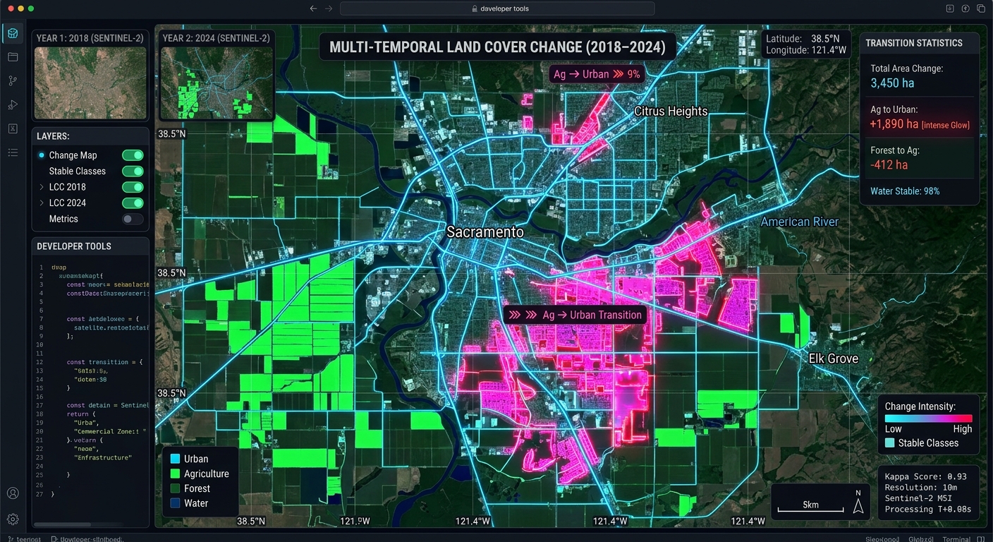
Multi-Temporal Remote Sensing Change Detection Using Google Earth Engine and Random Forest Classifiers
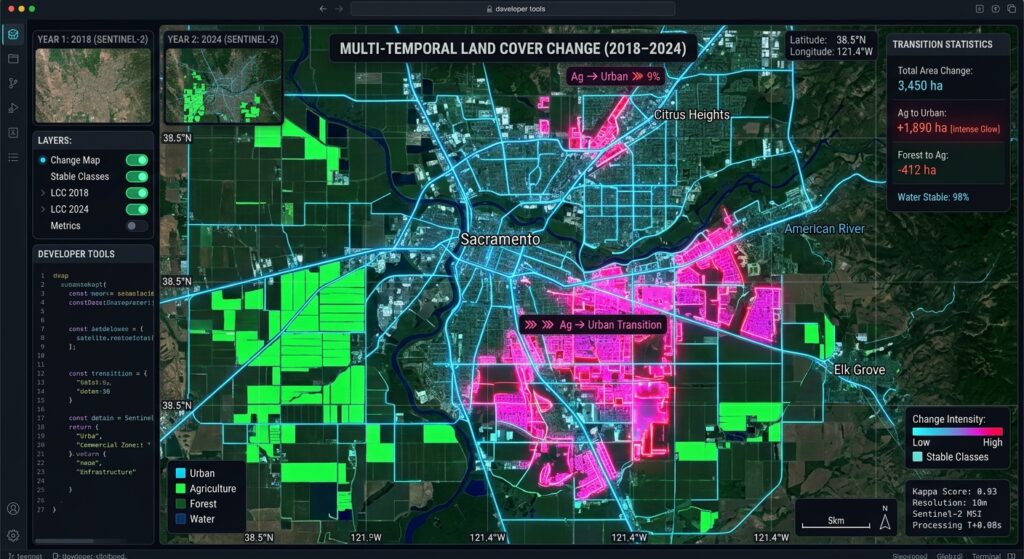
Monitoring landscape transformations over decadal timescales requires moving beyond simple spectral indices. Traditional bi-temporal approaches—such as manual image differencing or post-classification comparison using heuristic thresholds—frequently fall short when applied to complex, multi-year land-use and land-cover (LULC) change detection. Factors like inter-annual phenological variations, illumination geometry differences, atmospheric artifacts, and sensor calibration shifts often introduce noise that thresholding alone cannot reliably isolate.
To automate and scale robust LULC monitoring, remote sensing analysts leverage cloud-native geospatial platforms like Google Earth Engine (GEE) paired with non-parametric machine learning algorithms. In this advanced tutorial, we will construct an end-to-end multi-temporal classification and change detection pipeline using Sentinel-2 imagery, spectral-temporal metrics, and
ee.Classifier.smileRandomForest.The Limitations of Traditional Image Differencing
Traditional change detection relies heavily on bi-temporal spectral change vector analysis (CVA) or normalized difference vegetation index (NDVI) differencing between two static dates. While computationally lightweight, these methods suffer from several critical bottlenecks:
-
Phenological Mismatches: Comparing an image acquired during the dry season in a baseline year with one from the wet season in a target year produces false positives driven by seasonal vegetation flushes rather than true land conversion.
-
Atmospheric and Illumination Residuals: Uncorrected sub-pixel haze, aerosol optical depth variations, and topographic shadow shifts alter surface reflectance values independently of land cover alterations.
-
Class-Blind Outputs: Simple raster differencing flags where spectral changes occurred but provides no semantic context regarding what transition took place (e.g., distinguishing between forest-to-agriculture conversion versus agricultural fallow cycles).
By implementing a supervised classification workflow across multiple dates using multi-spectral feature spaces, we assign explicit semantic labels to each pixel per epoch, enabling precise transition matrix generation and error tracking.
Setting Up in Google Earth Engine
Our workflow is implemented using the Google Earth Engine JavaScript API. The pipeline processes Sentinel-2 Level-2A (Bottom-Of-Atmosphere reflectance) collections, constructs median composite mosaics, extracts spectral and textural feature spaces, trains an ensemble Random Forest classifier, and evaluates categorical transitions between baseline and target epochs.
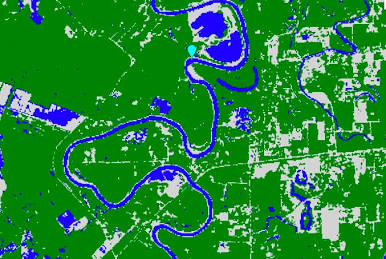
Step 1: Multi-Temporal Remote Sensing Change Detection Using Google Earth Engine and Random Forest Classifiers
To mitigate phenological noise, we construct annual median composites filtered by cloud probability and scene classification layers (SCL). We also compute standard spectral indices—such as NDVI, NDWI, and NDBI—to enhance separability between vegetation, water bodies, and built-up infrastructure.
JavaScript
// Define Study Area Region of Interest (ROI)
var roi = ee.Geometry.Polygon([[
  [36.65, -1.35],
  [36.85, -1.35],
  [36.85, -1.20],
  [36.65, -1.20]
]]);

Map.centerObject(roi, 11);

// Cloud Masking Function for Sentinel-2 MSI Level-2A
function maskS2clouds(image) {
  var qa = image.select('QA60');
  var cloudBitMask = 1 << 10;
  var cirrusBitMask = 1 << 11;
  var mask = qa.bitwiseAnd(cloudBitMask).eq(0)
    .and(qa.bitwiseAnd(cirrusBitMask).eq(0));

  // Optional: Use Scene Classification Layer (SCL) to remove clouds/shadows
  var scl = image.select('SCL');
  var nonWaterMask = scl.neq(3).and(scl.neq(8)).and(scl.neq(9)).and(scl.neq(10));

  return image.updateMask(mask.and(nonWaterMask))
    .divide(10000) // Scale factor to surface reflectance
    .copyProperties(image, ['system:time_start']);
}

// Function to add spectral indices for feature enhancement
function addIndices(image) {
  var ndvi = image.normalizedDifference(['B8', 'B4']).rename('NDVI');
  var ndwi = image.normalizedDifference(['B3', 'B8']).rename('NDWI');
  var ndbi = image.normalizedDifference(['B11', 'B8']).rename('NDBI');
  var bsi = image.expression(
    '((SWIR + Red) - (NIR + Blue)) / ((SWIR + Red) + (NIR + Blue))', {
      'SWIR': image.select('B11'),
      'Red': image.select('B4'),
      'NIR': image.select('B8'),
      'Blue': image.select('B2')
    }).rename('BSI');

  return image.addBands([ndvi, ndwi, ndbi, bsi]);
}

// Composite builder for a given year
function getAnnualComposite(year, geometry) {
  var startDate = ee.Date.fromYMD(year, 1, 1);
  var endDate = ee.Date.fromYMD(year, 12, 31);

  var collection = ee.ImageCollection('COPERNICUS/S2_SR_HARMONIZED')
    .filterBounds(geometry)
    .filterDate(startDate, endDate)
    .filter(ee.Filter.lt('CLOUDY_PIXEL_PERCENTAGE', 20))
    .map(maskS2clouds)
    .map(addIndices);

  return collection.median().clip(geometry);
}

// Generate Baseline (2018) and Target (2025) Composites
var bands = ['B2', 'B3', 'B4', 'B8', 'B11', 'B12', 'NDVI', 'NDWI', 'NDBI', 'BSI'];
var baselineImage = getAnnualComposite(2018, roi).select(bands);
var targetImage = getAnnualComposite(2025, roi).select(bands);

// Visualize Baseline Composite (False Color Infrared: NIR, Red, Green)
Map.addLayer(baselineImage, {bands: ['B8', 'B4', 'B3'], min: 0.05, max: 0.4}, 'Baseline Composite 2018');
Map.addLayer(targetImage, {bands: ['B8', 'B4', 'B3'], min: 0.05, max: 0.4}, 'Target Composite 2025');
Step 2: Collecting Training Samples for Distinct Land Cover Classes
For supervised classification, we define four core land cover classes:
-
1: Water (rivers, reservoirs, wetlands)
-
2: Forest / Dense Vegetation (natural canopy, closed thickets)
-
3: Agriculture / Grassland (croplands, pastures, fallow fields)
-
4: Built-up / Urban (impermeable surfaces, concrete, industrial zones)
For rigorous cross-temporal consistency, training points must ideally represent stable reference features across both epochs, or be collected independently per year using stratified random sampling over high-resolution historical reference imagery (e.g., Google Earth Time Machine).
JavaScript
// Simulated FeatureCollection representing training polygons
// In practice, these are digitized or imported from verified reference datasets
var waterPoints = ee.FeatureCollection([
  ee.Feature(ee.Geometry.Point([36.72, -1.28]), {class: 1}),
  ee.Feature(ee.Geometry.Point([36.71, -1.27]), {class: 1})
]);

var forestPoints = ee.FeatureCollection([
  ee.Feature(ee.Geometry.Point([36.68, -1.22]), {class: 2}),
  ee.Feature(ee.Geometry.Point([36.69, -1.23]), {class: 2})
]);

var agPoints = ee.FeatureCollection([
  ee.Feature(ee.Geometry.Point([36.80, -1.30]), {class: 3}),
  ee.Feature(ee.Geometry.Point([36.82, -1.31]), {class: 3})
]);

var urbanPoints = ee.FeatureCollection([
  ee.Feature(ee.Geometry.Point([36.78, -1.26]), {class: 4}),
  ee.Feature(ee.Geometry.Point([36.77, -1.25]), {class: 4})
]);

var trainingSamples = waterPoints.merge(forestPoints).merge(agPoints).merge(urbanPoints);

// Extract training values from baseline and target imagery
var baselineTrainingData = baselineImage.sampleRegions({
  collection: trainingSamples,
  properties: ['class'],
  scale: 10,
  tileScale: 4
});

var targetTrainingData = targetImage.sampleRegions({
  collection: trainingSamples,
  properties: ['class'],
  scale: 10,
  tileScale: 4
});
Step 3: Training the ee.Classifier.smileRandomForest Model
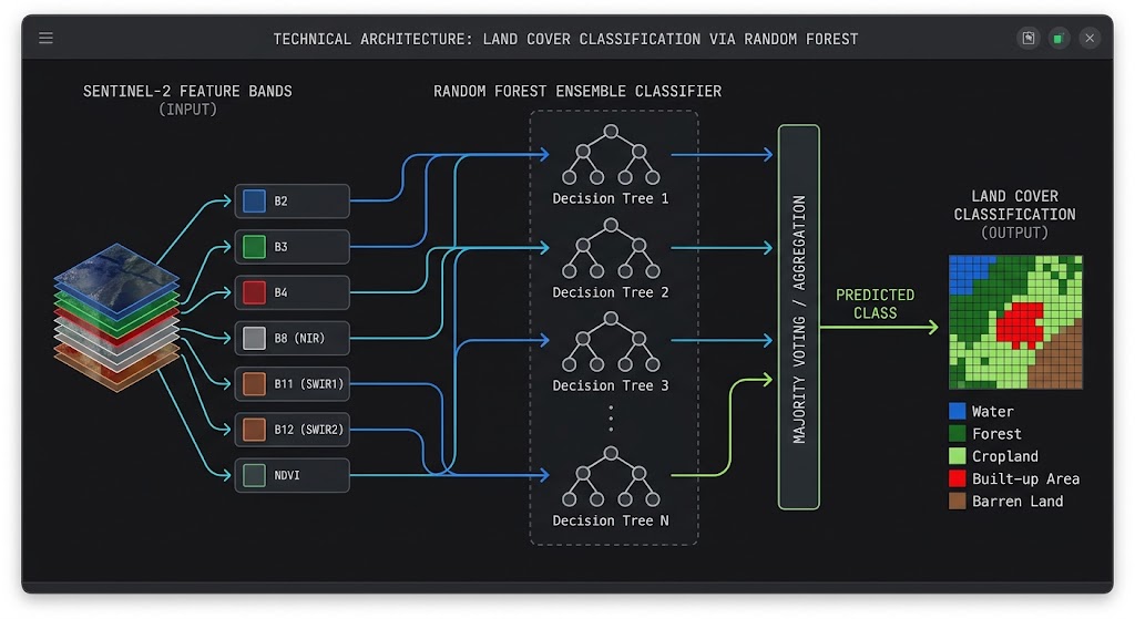
Random Forest classifiers excel in remote sensing applications due to their resistance to overfitting, handling of high-dimensional feature spaces, and ability to process non-linear spectral responses. We train two independent classifiers for our baseline and target composites to account for slight radiometric calibration variance between years, or train a single joint classifier if feature normalization is applied.
JavaScript
// Configure Random Forest Classifier with 100 decision trees
var numberOfTrees = 100;
var rfClassifier = ee.Classifier.smileRandomForest(numberOfTrees)
  .setOutputMode('CLASSIFICATION');

// Train Baseline Classifier (2018)
var trainedBaselineClassifier = rfClassifier.train({
  features: baselineTrainingData,
  classProperty: 'class',
  inputProperties: bands
});

// Train Target Classifier (2025)
var trainedTargetClassifier = rfClassifier.train({
  features: targetTrainingData,
  classProperty: 'class',
  inputProperties: bands
});

// Classify Baseline and Target Imagery
var classifiedBaseline = baselineImage.classify(trainedBaselineClassifier).rename('classification_2018');
var classifiedTarget = targetImage.classify(trainedTargetClassifier).rename('classification_2025');

// Visualization Palette for LULC Classes
var lulcPalette = [
  '1f77b4', // 1: Water (Blue)
  '2ca02c', // 2: Forest (Green)
  'bcbd22', // 3: Agriculture (Yellow/Brown)
  'd62728'  // 4: Built-up (Red)
];

Map.addLayer(classifiedBaseline, {min: 1, max: 4, palette: lulcPalette}, 'LULC 2018');
Map.addLayer(classifiedTarget, {min: 1, max: 4, palette: lulcPalette}, 'LULC 2025');
Step 4: Exporting Classified Raster Layers and Computing Transition Matrices
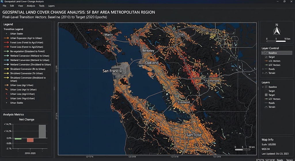
To quantify net and gross changes between 2018 and 2025, we combine the two classification rasters into a single change-vector image. By multiplying the baseline raster by 10 and adding the target raster, each unique pixel value corresponds to a specific land-cover transition path (e.g., code
24 indicates a transition from Forest 2 to Built-up 4).JavaScript
// Combine baseline and target classifications into a single change raster
// Formula: Change Code = (Class_2018 * 10) + Class_2025
var changeRaster = classifiedBaseline.multiply(10).add(classifiedTarget).rename('transition_code');

// Visualize Transition Map
Map.addLayer(changeRaster, {min: 11, max: 44, palette: 'gray'}, 'Transition Matrix Raster');

// Compute Transition Area Statistics (Hectares)
var areaImage = ee.Image.pixelArea().divide(10000).addBands(changeRaster);

var transitionStats = areaImage.reduceRegion({
  reducer: ee.Reducer.sum().group({
    groupField: 1,
    groupName: 'transition_code'
  }),
  geometry: roi,
  scale: 10,
  maxPixels: 1e9
});

print('Transition Area Statistics (Hectares):', transitionStats);

// Export Classified Rasters to Google Drive
Export.image.toDrive({
  image: classifiedBaseline,
  description: 'LULC_Classification_2018',
  folder: 'EarthEngine_Exports',
  region: roi,
  scale: 10,
  maxPixels: 1e9
});

Export.image.toDrive({
  image: classifiedTarget,
  description: 'LULC_Classification_2025',
  folder: 'EarthEngine_Exports',
  region: roi,
  scale: 10,
  maxPixels: 1e9
});

Export.image.toDrive({
  image: changeRaster,
  description: 'LULC_Transition_Matrix_2018_2025',
  folder: 'EarthEngine_Exports',
  region: roi,
  scale: 10,
  maxPixels: 1e9
});
Advanced Analytical Considerations & Error Mitigation
While Random Forest supervised classification combined with cloud-free median composites resolves many traditional spectral discrepancies, production-grade change detection pipelines require careful attention to several residual error sources:
-
Topographic Illumination Effects: In rugged terrain, differential solar illumination alters apparent surface reflectance. Incorporating a Digital Elevation Model (DEM) like SRTM or NASADEM as an input feature during model training helps the Random Forest classifier account for slope and aspect effects.
-
Mixed Pixel Boundaries: Transition zones between urban sprawl and agricultural plots frequently suffer from mixed-pixel spectral blending. Applying morphological filters (such as modal smoothing or focal majority filters) helps remove salt-and-pepper classification noise.
-
Temporal Sampling Bias: Training samples must accurately reflect spectral variance across the entire study area. Relying exclusively on localized training patches can lead to spatial extrapolation errors when classifying heterogeneous regional landscapes.
For further exploration of time-series workflows, refer to our related guides on GEE Python time-series analysis and automated Principal Component Analysis on satellite bands to reduce dimensionality before classification.
Summary
Automating multi-temporal remote sensing change detection in Google Earth Engine using Random Forest classifiers provides a scalable, repeatable framework for monitoring environmental and urban dynamics. By combining robust cloud-masking protocols, multi-spectral index feature engineering, ensemble machine learning, and pixel-level transition matrix modeling, analysts can transition from subjective visual interpretations to rigorous, reproducible quantitative geographic assessments.