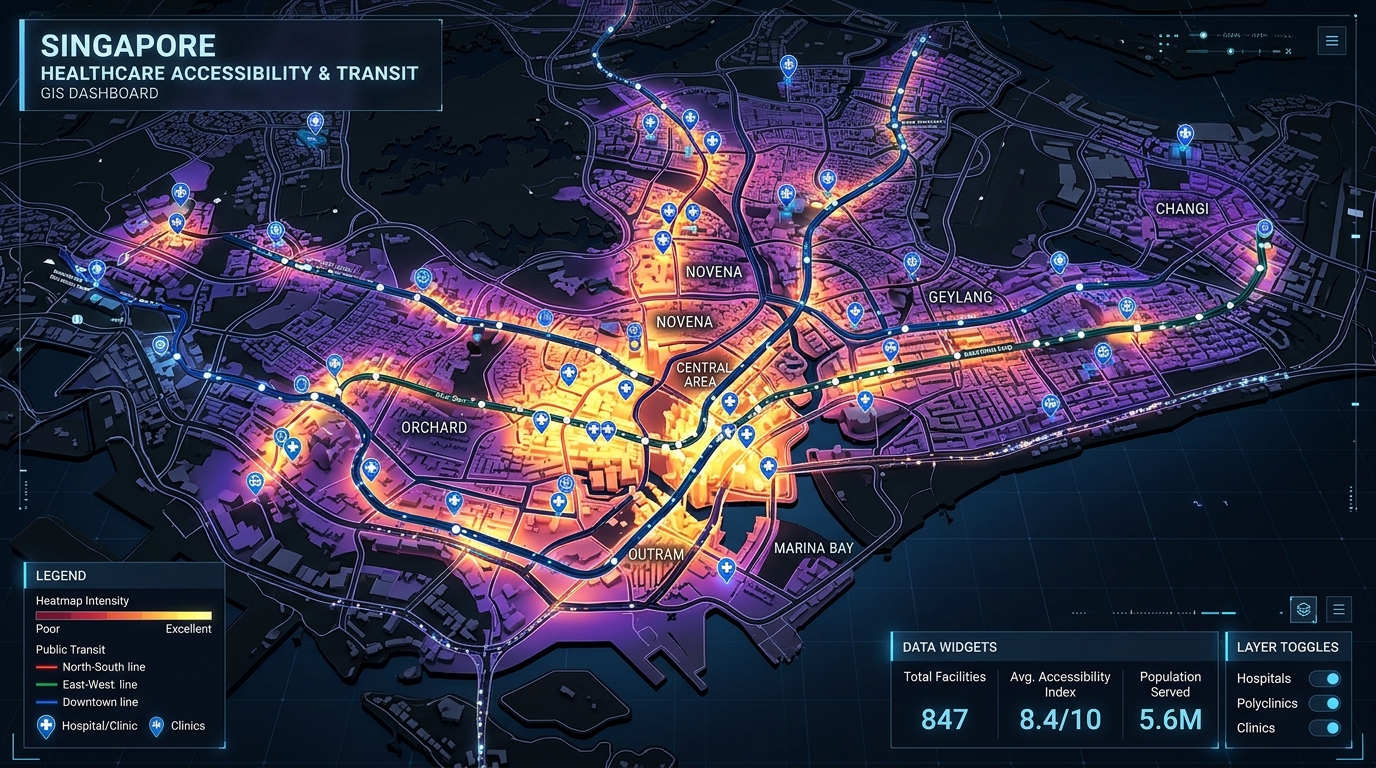
Analyzing Urban Healthcare Deserts: Measuring Spatial Mismatch and Accessibility Gaps

Introduction to Analyzing Urban Healthcare Deserts: Measuring Spatial Mismatch and Accessibility Gaps

A hospital can be geographically close to a neighborhood without being practically accessible to its residents. A clinic may be located two kilometers away, yet reaching it could require multiple public transport transfers, a long walk, or an expensive journey across a congested city. Meanwhile, a well-served commercial district may have several competing healthcare providers within a short travel time.

These inequalities raise an important urban planning question: Where are healthcare resources located relative to the populations that need them, and which communities face the greatest barriers to obtaining care?

Geographic Information Systems (GIS) provide a framework for answering this question through spatial accessibility analysis, network-based travel-time modeling, and demographic vulnerability assessment.

A healthcare desert is commonly used to describe an area where access to necessary health services is inadequate. However, the term does not have one universally applicable spatial definition. Researchers must specify which services are being studied, the acceptable travel time, the available provider capacity, and the population at risk.

Two concepts are especially important:

• Spatial accessibility: How easily a population can reach healthcare services, considering travel costs, facility availability, and competition for resources.
• Social vulnerability: The socioeconomic and demographic circumstances that may make people more susceptible to poor health outcomes or less able to overcome barriers to care.

Mapping these dimensions separately and then examining their intersection reveals more than a simple map of hospital locations.

This guide explains how to analyze urban healthcare deserts using GIS, with particular attention to the Two-Step Floating Catchment Area (2SFCA) method. It covers data preparation, network travel-time matrices, Python implementation, vulnerability mapping, and the implications for urban health policy.

1. Why Straight-Line Distance Is an Inadequate Measure of Healthcare Access

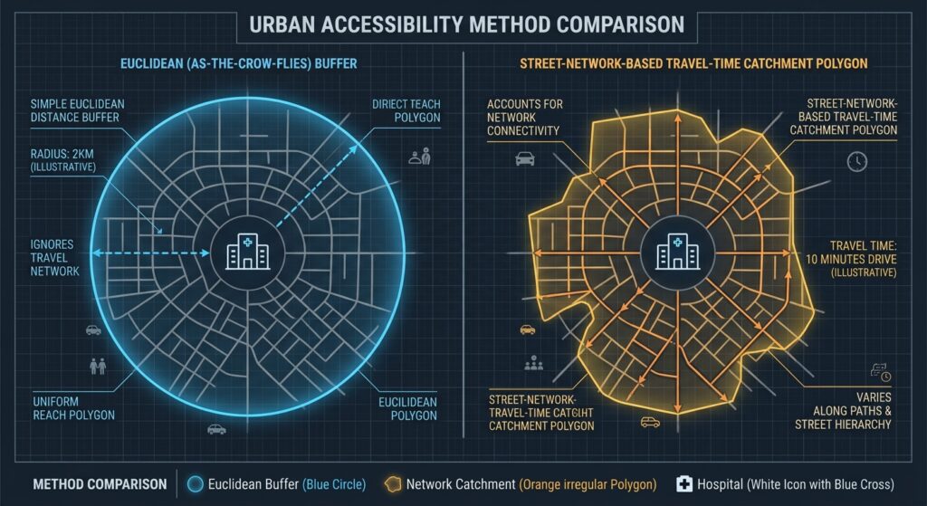
A conventional proximity analysis might draw a circular buffer around every hospital and identify census areas outside those circles. Although useful for preliminary screening, this method assumes that distance represents accessibility equally in every direction.

Urban geography rarely works that way.

Major highways can separate nearby neighborhoods from hospitals. Railways, rivers, fenced properties, restricted pedestrian crossings, and missing sidewalks can force people to take longer routes. Public transport users may encounter additional waiting times, service gaps, and transfers.

Travel times also vary by transportation mode and time of day. A ten-minute car journey does not necessarily translate into a ten-minute walk or bus trip.

A healthcare accessibility mapping tutorial should therefore distinguish between three common approaches.

Method	What it measures	Main limitation
Euclidean distance	Straight-line distance between locations	Ignores street layout and travel barriers
Network travel time	Estimated time to travel along a transport network	Depends on network quality, routing assumptions, and travel mode
Supply-demand accessibility	Reachable healthcare capacity relative to competing population demand	Requires provider capacity, population, and catchment assumptions

The third approach is especially important because reaching a facility does not guarantee access to its services. One hospital might have enough staff and appointment capacity for its catchment population, while another might be severely overstretched.

The World Health Organization’s AccessMod framework illustrates how GIS can assess physical accessibility, geographic coverage, and health-service capacity to support health system planning.

For a robust urban healthcare study, network travel time and supply-demand accessibility should be treated as complementary measures rather than competing alternatives.

2. Methodological Deep Dive: The Two-Step Floating Catchment Area Method

The Two-Step Floating Catchment Area method provides a practical way to measure potential spatial access by combining healthcare supply, population demand, and travel-time thresholds.

Unlike a simple facility count, 2SFCA accounts for the fact that several communities may depend on the same healthcare provider.

Step 1: Calculate provider-to-population ratios

For each healthcare facility (j), identify every population location (i) that falls within the facility’s travel-time catchment.

Define the provider-to-population ratio as:

[
R_j = \frac{S_j}{\sum_{i:d_{ij}\leq d_0} P_i}
]

Where:

• (R_j) is the supply-demand ratio for facility (j).
• (S_j) is its available service capacity.
• (P_i) is the population at demand location (i).
• (d_{ij}) is the network travel time between population location (i) and facility (j).
• (d_0) is the maximum acceptable travel time.

Suppose a clinic can provide 100 units of a relevant service per week and serves 5,000 people within its 30-minute catchment.

Its provider-to-population ratio is:

[
R_j = \frac{100}{5000}=0.02
]

This represents 0.02 units of weekly service capacity per person in the catchment, assuming the capacity and population figures are comparable to the demand being modeled.

The interpretation of (S_j) matters. Depending on the analysis, supply may be represented by clinicians, full-time-equivalent staff, appointment slots, or service-specific capacity. Provider counts alone are a weak proxy when facilities differ substantially in size.

Step 2: Calculate accessibility for each population location

For each demand location (i), find all facilities accessible within the same travel-time threshold and sum their supply-demand ratios.

[
A_i = \sum_{j:d_{ij}\leq d_0} R_j
]

The resulting (A_i) measures potential spatial access at location (i). Larger values indicate greater available healthcare capacity relative to population demand under the model’s assumptions.

If supply is measured in providers and demand in people, multiply the score by 1,000 to express it as providers per 1,000 population.

The 2SFCA method is widely used in spatial accessibility research because it accommodates overlapping catchments and incorporates competition for healthcare resources. However, standard 2SFCA treats all locations inside a catchment equally and all locations outside it as inaccessible. These limitations are discussed in the systematic methodological review of healthcare accessibility models.

An important extension: Enhanced 2SFCA

Enhanced 2SFCA (E2SFCA) addresses the abrupt boundaries of the basic model by assigning lower weights to locations with longer travel times.

For example, researchers might use the following illustrative weights:

Travel time	Weight
0–10 minutes	1.0
More than 10–20 minutes	0.6
More than 20–30 minutes	0.3
More than 30 minutes	0.0

The provider ratio becomes:

[
R_j = \frac{S_j}{\sum_i P_i w(d_{ij})}
]

And population accessibility becomes:

[
A_i = \sum_j R_j w(d_{ij})
]

Here, (w(d_{ij})) represents the travel-time decay weight. The weights should reflect the study’s assumptions and, where possible, observed healthcare-seeking behavior.

This extension is particularly useful in cities where small differences in travel time can substantially influence service use. More advanced variants can also account for facility-specific catchments, multiple transportation modes, and time-dependent accessibility.

3. Step One: Prepare Population and Healthcare Facility Data

A spatial mismatch analysis begins with two datasets: population demand and healthcare supply.

Population demand data

Suitable demand units include census tracts, census block groups, administrative neighborhoods, or population grid cells.

Useful attributes include:

• Total population and population density.
• Household income or poverty measures.
• Household vehicle ownership.
• Population aged 65 and older.
• Disability-related indicators and other locally relevant vulnerability measures.

Demand units should represent where people live rather than simply where administrative centroids happen to fall. For large or irregular census polygons, population-weighted centroids or gridded population estimates may better represent the distribution of residents.

Healthcare supply data

Create a point dataset containing hospitals, primary healthcare centers, outpatient clinics, or other relevant facilities.

Recommended attributes include a unique facility ID, coordinates, facility type, operating status, service capacity, and the specific services offered.

Different service types should usually be modeled separately. A nearby pharmacy does not substitute for a hospital offering emergency surgery, just as a general clinic may not provide specialist oncology care.

The WHO Geolocated Health Facilities Data initiative highlights the importance of maintaining accurate, georeferenced health facility inventories and consistent facility identifiers.

Before calculating accessibility, verify the location accuracy of each facility and remove or correct duplicate, inactive, or incorrectly classified records.

4. Step Two: Generate Origin-Destination Travel-Time Matrices

The origin-destination (OD) matrix connects each population location to the healthcare facilities it could potentially reach.

Every useful OD record should identify an origin, destination, and estimated travel time.

demand_id	provider_id	travel_min
T001	H001	8.4
T001	H002	17.2
T002	H001	24.6
T002	H002	12.1

These values are illustrative. The matrix should contain travel times calculated from the actual street or transit network, not distances inferred from geographic proximity.

Building the travel-time matrix

Several workflows are possible.

Desktop GIS: ArcGIS Network Analyst provides an OD Cost Matrix solver that calculates travel costs between origins and destinations along a network. See the ArcGIS Pro OD Cost Matrix documentation.

Open-source routing: A routing engine such as OpenTripPlanner can model public transport journeys by combining transit schedules with walking connections and a suitable pedestrian network.

Public transport analysis: General Transit Feed Specification (GTFS) data provide information about transit routes, stops, trips, and schedules. The official GTFS documentation describes the standard.

GTFS schedules alone do not generate door-to-door travel times. They must be combined with a routing engine and appropriate access, transfer, and egress assumptions.

For a public transport accessibility study, consider walking time to the first stop, waiting time, scheduled journey time, transfer penalties, and walking time from the last stop to the facility. Analyze a defined service period because the available routes and journey times can differ considerably between morning peaks, evenings, weekends, and public holidays.

Set the catchment threshold

For a metropolitan primary-care study, a 30-minute travel-time threshold might be a useful starting assumption. Specialist hospitals may require a different threshold.

Do not assume that one threshold is appropriate for every city, service type, or population group. Test alternative thresholds and report how sensitive the results are to those choices.

To control the size of the matrix, retain only reachable origin-destination pairs within the maximum threshold required by the analysis. This reduces memory use and avoids storing unnecessary routes.

5. Step Three: Calculate 2SFCA Accessibility with Python

The following implementation calculates the basic 2SFCA score from an OD travel-time table. It uses pandas and NumPy, making it easy to integrate the results into a GeoPandas workflow.

Install the relevant packages:

pip install pandas numpy geopandas matplotlib

Prepare three CSV files:

• demand.csv containing demand_id, population, and optionally vulnerability variables.
• providers.csv containing provider_id and capacity.
• od_times.csv containing demand_id, provider_id, and travel_min.

The example assumes that all facility capacity values measure the same type of service and are appropriate to compare with the population demand.

import numpy as np
import pandas as pd

# Load datasets.
demand = pd.read_csv("demand.csv")
providers = pd.read_csv("providers.csv")
od = pd.read_csv("od_times.csv")

# Basic input validation.
required_demand = {"demand_id", "population"}
required_providers = {"provider_id", "capacity"}
required_od = {"demand_id", "provider_id", "travel_min"}

if not required_demand.issubset(demand.columns):
    raise ValueError("Missing required demand columns.")

if not required_providers.issubset(providers.columns):
    raise ValueError("Missing required provider columns.")

if not required_od.issubset(od.columns):
    raise ValueError("Missing required OD columns.")

if demand["demand_id"].duplicated().any():
    raise ValueError("demand_id must be unique.")

if providers["provider_id"].duplicated().any():
    raise ValueError("provider_id must be unique.")

if (demand["population"] < 0).any():
    raise ValueError("Population cannot be negative.")

if (providers["capacity"] < 0).any():
    raise ValueError("Capacity cannot be negative.")

# Use a 30-minute travel-time catchment.
cutoff = 30.0

od["travel_min"] = pd.to_numeric(
    od["travel_min"], errors="raise"
)

if not np.isfinite(od["travel_min"]).all():
    raise ValueError("OD travel times must be finite.")

# Remove duplicate origin-destination pairs.
if od.duplicated(["demand_id", "provider_id"]).any():
    raise ValueError("Duplicate OD pairs must be resolved.")

# Restrict analysis to valid, reachable pairs.
od = od[
    (od["travel_min"] >= 0)
    & (od["travel_min"] <= cutoff)
].copy()

# Attach population to each OD record.
od = od.merge(
    demand[["demand_id", "population"]],
    on="demand_id",
    how="left",
    validate="many_to_one"
)

# Attach healthcare capacity to each OD record.
od = od.merge(
    providers[["provider_id", "capacity"]],
    on="provider_id",
    how="left",
    validate="many_to_one"
)

if od[["population", "capacity"]].isna().any().any():
    raise ValueError("OD matrix contains unmatched IDs.")

# STEP 1: Calculate population within each provider's catchment.
catchment_population = (
    od.groupby("provider_id")["population"]
    .sum()
    .rename("catchment_population")
)

provider_ratios = providers.join(
    catchment_population,
    on="provider_id"
)

provider_ratios["catchment_population"] = (
    provider_ratios["catchment_population"].fillna(0)
)

# Capacity per person within the catchment.
provider_ratios["R_j"] = np.divide(
    provider_ratios["capacity"],
    provider_ratios["catchment_population"],
    out=np.zeros(len(provider_ratios), dtype=float),
    where=provider_ratios["catchment_population"].to_numpy() > 0
)

# STEP 2: Sum the ratios of reachable providers for each origin.
od = od.merge(
    provider_ratios[["provider_id", "R_j"]],
    on="provider_id",
    how="left",
    validate="many_to_one"
)

accessibility = (
    od.groupby("demand_id")["R_j"]
    .sum()
    .rename("access_per_person")
)

demand = demand.join(
    accessibility,
    on="demand_id"
)

demand["access_per_person"] = (
    demand["access_per_person"].fillna(0)
)

# Express capacity as units per 1,000 population.
demand["access_per_1000"] = (
    demand["access_per_person"] * 1000
)

demand.to_csv("healthcare_accessibility.csv", index=False)

print(demand[
    ["demand_id", "access_per_1000"]
].head())

The output contains a continuous accessibility score for every demand location. Locations with no reachable providers receive zero under this model.

A few details deserve attention. First, the code assumes a complete set of reachable pairs within the cutoff; a missing OD record should not be interpreted as a valid route unless the routing workflow confirms that no acceptable route exists. Second, supply capacity and population demand must refer to compatible units. Third, the basic calculation does not account for travel-time decay within the catchment.

Extending the code to E2SFCA

To incorporate the illustrative distance-decay weights, assign a weight to every reachable OD pair:

def travel_weight(minutes):
    if minutes <= 10:
        return 1.0
    elif minutes <= 20:
        return 0.6
    elif minutes <= 30:
        return 0.3
    return 0.0

od["weight"] = od["travel_min"].apply(travel_weight)

For this extended model, replace the Step 1 denominator with the weighted demand:

od["weighted_population"] = (
    od["population"] * od["weight"]
)

weighted_demand = (
    od.groupby("provider_id")["weighted_population"]
    .sum()
    .rename("weighted_population")
)

provider_ratios = providers.join(
    weighted_demand,
    on="provider_id"
)

provider_ratios["weighted_population"] = (
    provider_ratios["weighted_population"].fillna(0)
)

provider_ratios["R_j"] = np.divide(
    provider_ratios["capacity"],
    provider_ratios["weighted_population"],
    out=np.zeros(len(provider_ratios), dtype=float),
    where=provider_ratios["weighted_population"].to_numpy() > 0
)

Then calculate accessibility by summing R_j * weight for each demand location:

od = od.drop(columns=["R_j"], errors="ignore").merge(
    provider_ratios[["provider_id", "R_j"]],
    on="provider_id",
    how="left",
    validate="many_to_one"
)

accessibility = (
    (od["R_j"] * od["weight"])
    .groupby(od["demand_id"])
    .sum()
)

demand["access_per_person_e2sfca"] = (
    demand["demand_id"]
    .map(accessibility)
    .fillna(0)
)

demand["access_per_1000_e2sfca"] = (
    demand["access_per_person_e2sfca"] * 1000
)

This calculation implements a simple distance-decay 2SFCA variant. Because the weights change the denominator in Step 1 and the accessibility sum in Step 2, the resulting scores should not be interpreted as directly interchangeable with the unweighted 2SFCA values.

6. Step Four: Measure Spatial Mismatch and Demographic Vulnerability

Low accessibility identifies areas with relatively limited healthcare supply, but it does not automatically establish which communities face the greatest disadvantage.

A second analytical layer should capture the characteristics of residents who may have more difficulty reaching or paying for care.

Potential indicators include:

• High poverty or low median household income.
• High proportions of households without access to a vehicle.
• Large older-adult populations.
• High disability prevalence.
• Other relevant measures of socioeconomic disadvantage.

In the United States, the CDC/ATSDR Social Vulnerability Index provides census-based indicators and composite vulnerability measures. Outside the United States, use comparable local census variables or a locally appropriate vulnerability index instead of treating the CDC index as universally applicable.

Identify priority areas using quantiles

A useful screening method is to identify census areas that simultaneously fall within the lowest accessibility quartile and the highest vulnerability quartile.

For example:

access_q25 = demand["access_per_1000"].quantile(0.25)
vulnerability_q75 = demand["svi"].quantile(0.75)

demand["low_access"] = (
    demand["access_per_1000"] <= access_q25
)

demand["high_vulnerability"] = (
    demand["svi"] >= vulnerability_q75
)

demand["healthcare_desert_priority"] = (
    demand["low_access"]
    & demand["high_vulnerability"]
)

Here, svi is assumed to be a consistently oriented score in which higher values indicate greater vulnerability. Check the definition of any composite index before applying this rule.

This is a relative screening method, not a universal definition of a healthcare desert. Its results depend on the study area and the selected quantiles. A city in which nearly every neighborhood has poor access may still have areas that rank in the top accessibility quartile without providing adequate care.

Where absolute standards exist, also report the proportion of the population beyond a specified travel-time threshold and the proportion below a defined service-capacity target.

Map the overlap with GeoPandas

Join the accessibility results to census polygons using a stable geographic identifier.

import geopandas as gpd
import matplotlib.pyplot as plt

tracts = gpd.read_file("census_areas.gpkg")

tracts = tracts.merge(
    demand[
        [
            "demand_id",
            "access_per_1000",
            "svi",
            "healthcare_desert_priority"
        ]
    ],
    left_on="tract_id",
    right_on="demand_id",
    how="left",
    validate="one_to_one"
)

fig, ax = plt.subplots(figsize=(10, 8))

tracts.plot(
    column="healthcare_desert_priority",
    cmap="OrRd",
    legend=True,
    missing_kwds={
        "color": "lightgrey",
        "label": "Missing data"
    },
    ax=ax
)

ax.set_title(
    "Potential Healthcare Desert Priority Areas"
)
ax.set_axis_off()

plt.tight_layout()
plt.savefig(
    "healthcare_desert_hotspots.png",
    dpi=200
)
plt.show()

This map identifies census areas meeting both screening conditions. For a publication-quality analysis, create a bivariate choropleth with separate categories for low and high accessibility and vulnerability, enabling readers to distinguish high-vulnerability neighborhoods with good access from neighborhoods experiencing both disadvantages.

Image 1 placeholder: Bivariate map showing low spatial access overlaid with high social vulnerability census tracts

Alt text: Bivariate choropleth map highlighting urban healthcare deserts where high demographic vulnerability intersects with low 30-minute travel time access to medical facilities.

Image 2 placeholder: Diagram comparing straight-line buffer access versus network travel-time 2SFCA catchment accessibility

Alt text: Methodological visual comparing Euclidean straight-line buffer coverage with realistic street-network travel time catchment areas for health access analysis.

Add spatial statistics to strengthen hotspot detection

A bivariate map helps identify priority neighborhoods, but neighboring census areas are often geographically correlated.

Global Moran’s I can help assess whether accessibility values show overall spatial clustering. Local Moran’s I or Getis-Ord Gi* can identify statistically significant clusters or hotspots, depending on the chosen spatial weights and hypothesis.

For healthcare planning, particularly relevant clusters include neighborhoods with low access surrounded by other low-access areas and communities with persistently high vulnerability. Use a stated spatial weights definition, consider multiple-testing corrections for local statistics, and avoid interpreting statistical significance as proof of causation.

7. Policy and Urban Planning Implications

Healthcare accessibility maps are most useful when they guide a practical decision.

Mobile clinics and outreach services: Prioritize underserved neighborhoods where fixed facilities are distant, transport options are limited, or demand is high relative to available capacity.

New clinic locations: Use location-allocation analysis to evaluate candidate sites and identify locations that could improve population coverage rather than simply placing new facilities where land is inexpensive or demand is already well served.

Public transport investment: Improve the connectivity of neighborhoods whose network travel times remain high despite their geographic proximity to existing hospitals.

Capacity expansion: Distinguish areas suffering from long travel times from areas where nearby facilities are overloaded. These require different interventions: transport or facility-location changes in one case, capacity or staffing improvements in the other.

Equity monitoring: Repeat the analysis as populations change, facilities open or close, and transportation infrastructure develops. Compare different demographic groups where reliable data permit, while protecting sensitive information.

A documented example comes from research on geographic accessibility to public and private health facilities in Kenya. The study combined an updated geocoded inventory with road networks, land cover, topography, travel barriers, and different transport modes to model access. It demonstrates why geographic accessibility analysis benefits from more realistic movement assumptions than simple circular buffers. See the 2021 Kenya health-facility accessibility study.

Importantly, an accessibility score is not a direct measure of realized healthcare use or quality. A facility may be geographically accessible but unaffordable, closed, understaffed, or unable to provide a required treatment. Planning decisions should therefore combine the GIS results with service availability, affordability, community consultation, and health-system evidence.

8. Methodological Limitations and Quality Assurance

Before publishing a healthcare desert map, document the assumptions that can alter its interpretation.

Facility capacity: If exact staffing, appointment, or service-capacity data are unavailable, state clearly when facility counts are being used as proxies.

Catchment thresholds: Compare multiple travel-time cutoffs and, where possible, validate them against observed service-use patterns.

Travel mode: Model walking, driving, and public transport separately when relevant. A map based on driving times may substantially misrepresent access for households without vehicles.

Boundary effects: Include facilities and population demand outside the study boundary when they could realistically serve the study population. City borders do not necessarily represent healthcare catchment boundaries.

Geographic aggregation: Census-tract results describe population areas, not every individual household. Large administrative units can conceal important local inequalities.

Temporal accuracy: Ensure that population estimates, road networks, public transport schedules, facility operations, and service capacities refer to compatible periods.

Model uncertainty: Conduct sensitivity analyses to determine whether priority areas remain underserved across plausible alternative assumptions.

These checks transform the analysis from a visually compelling map into a more defensible decision-support product.

9. SEO Interlinking and Further Reading

Suggested internal links:

• GTFS Network Routing and Public Transport Accessibility — explain schedule-based multimodal travel-time analysis.
• Spatial Statistics and Hotspot Analysis in GIS — cover spatial autocorrelation and local cluster detection.
• Choropleth Mapping Best Practices — explain classification methods, legends, uncertainty, and accessible cartographic design.

Replace these suggested paths with the corresponding live URLs on your website.

Recommended external references:

• WHO AccessMod — geographic healthcare accessibility and coverage analysis.
• WHO Geolocated Health Facilities Data — geospatial healthcare facility inventories.
• CDC/ATSDR Social Vulnerability Index — demographic vulnerability data and documentation for the United States.
• GTFS Official Documentation — public transportation schedules and data structures.
• Systematic Review of Healthcare Accessibility Methods — methodological developments in 2SFCA and related accessibility models.

Conclusion and Key Takeaways

Analyzing urban healthcare deserts requires more than measuring the distance between neighborhoods and hospitals. A robust spatial accessibility assessment must account for the transport network, travel time, available healthcare capacity, competing population demand, and the characteristics of communities facing barriers to care.

The Two-Step Floating Catchment Area method provides a practical foundation. By calculating provider-to-population ratios and summing the ratios of reachable facilities, analysts can compare potential healthcare access across census areas. Enhanced variants can incorporate distance decay, while demographic vulnerability indicators reveal where limited access intersects with socioeconomic disadvantage.

The resulting accessibility scores, network maps, and vulnerability overlays can support decisions about mobile clinics, facility expansion, transport improvements, and public health investment.

The central principle is to measure potential access realistically, identify inequities transparently, and validate GIS findings against the operational realities of the health system. A healthcare desert map is most valuable when it helps planners determine not only where access is poor, but also which intervention is most likely to improve it.