

Managing Spatio-Temporal Data Streams with Apache Kafka and PostGIS
Introduction: Managing Spatio-Temporal Data Streams Apache Kafka PostGIS

When implementing **Managing Spatio-Temporal Data Streams Apache Kafka PostGIS** pipelines, high-velocity, continuous telemetry streams present unique architectural challenges. High-velocity, continuous telemetry streams—such as connected vehicle location tracking, dynamic fleet management, mobile delivery platforms, and smart-city IoT sensor grids—present unique architectural challenges. Unlike static spatial data, spatio-temporal data streams possess a dual nature: heavy write traffic driven by continuous movement and complex multi-dimensional indexing needs across space ($x, y$) and time ($t$).
Processing hundreds of thousands of incoming GPS coordinates per second while offering real-time spatial query access requires decoupling data ingestion from persistent spatial storage. Simple point-in-time relational writes degrade quickly under concurrent streaming lock contention. Conversely, purely append-only log brokers lack out-of-the-box spatial indexing capabilities like $R$-trees or spatial bounding-box operators.
In this guide, we will design and build an enterprise-grade real-time ingestion pipeline using Apache Kafka as a high-throughput message broker, Python for streaming execution and geometry validation, and PostGIS for spatio-temporal persistence and indexed querying.
The Real-Time Architecture Stack
To balance low latency with horizontal scalability, we decouple event streaming, stream transformation, and spatial persistence.
[ IoT Sensors / Vehicles ]
          │
          │ JSON Telemetry Payload (MQTT/HTTP REST)
          ▼
┌───────────────────────────────────┐
│     Apache Kafka Ingestion        │
│   (Topic: vehicle-telemetry-raw)  │
└─────────────────┬─────────────────┘
                  │
                  ▼
┌───────────────────────────────────┐
│     Python Consumer Engine        │
│  - confluent-kafka (Async Read)   │
│  - Shapely (Geometry Validation)  │
│  - psycopg2 (Connection Pool)     │
└─────────────────┬─────────────────┘
                  │
                  ▼
┌───────────────────────────────────┐
│    PostGIS Spatial Storage        │
│  - Partitioned Point Track Table  │
│  - Upsert Live State Table        │
│  - GiST (R-Tree) Spatial Index    │
└───────────────────────────────────┘
[Image 1: Data flow pipeline architecture from IoT sensors through Apache Kafka to PostGIS]
Alt Text: “Architecture diagram showing real-time GPS telemetry streaming from IoT devices through Apache Kafka message queues into a PostGIS spatial database.”
Architectural Components
-
Apache Kafka Message Broker: Serves as the durable, fault-tolerant buffer for unstructured, incoming telemetry events. Partition keys based on unique device identifiers (e.g.,
vehicle_id) ensure strict time-series ordering per device. -
Python Stream Ingestion Layer: Consumes raw JSON events asynchronously via high-performance C bindings (
confluent-kafka), validates coordinate ranges, converts raw coordinates into WKT/EWKB geometries, and constructs batch parameters. -
PostGIS Spatial Database: Serves as the indexed target layer. It maintains historical track logs using time-range partitioning alongside GiST indexes while managing an optimized current-state lookup table.
Step 1: Configuring Kafka Topics for Raw GPS Payloads
When streaming spatial data, partition distribution is critical. Setting partition keys based on
vehicle_id guarantees that records from a given tracking unit land in the exact same partition, preserving timestamp sequence integrity without cross-partition coordination overhead.Creating the Kafka Topic
Execute the following administrative command using the Kafka cluster tools to create a dedicated telemetry topic with replication and retention policies tailored for stream ingestion:
Bash
kafka-topics.sh --create \
  --bootstrap-server localhost:9092 \
  --replication-factor 3 \
  --partitions 12 \
  --topic vehicle-telemetry-raw \
  --config cleanup.policy=delete \
  --config retention.ms=86400000 \
  --config segment.bytes=1073741824
JSON Telemetry Payload Schema
Below is the standard JSON structure expected from edge IoT sensors or HTTP gateways:
JSON
{
  "vehicle_id": "v-8942-kenya",
  "timestamp": "2026-10-23T09:15:30.104Z",
  "latitude": -1.26194,
  "longitude": 36.73222,
  "altitude_m": 1780.5,
  "speed_kmh": 48.2,
  "heading_deg": 142.5,
  "accuracy_m": 2.1
}
Step 2: Database Schema & Spatial Indexing in PostGIS
To achieve efficient read performance for spatial applications alongside high-rate write streams, the database structure employs two main design patterns:
-
Append-Only Historical Tracks: Declarative table partitioning by time, enabling quick index drops for data retention and minimizing index maintenance overhead.
-
Current State Table: An operational state table updated via spatial
UPSERTstatements for rapid key-value and bounding-box spatial lookups.
PostGIS Schema Definition
SQL
-- Enable PostGIS extension
CREATE EXTENSION IF NOT EXISTS postgis;

-- 1. Append-Only Historical Tracks Table
CREATE TABLE vehicle_telemetry_history (
    id BIGGENERATED ALWAYS AS IDENTITY,
    vehicle_id VARCHAR(64) NOT NULL,
    recorded_at TIMESTAMPTZ NOT NULL,
    geom GEOMETRY(PointZ, 4326) NOT NULL,
    speed_kmh REAL,
    heading_deg REAL,
    accuracy_m REAL,
    created_at TIMESTAMPTZ DEFAULT CURRENT_TIMESTAMP,
    PRIMARY KEY (recorded_at, vehicle_id, id)
) PARTITION BY RANGE (recorded_at);

-- Create initial monthly partition
CREATE TABLE vehicle_telemetry_h2026_10 PARTITION OF vehicle_telemetry_history
    FOR VALUES FROM ('2026-10-01 00:00:00+00') TO ('2026-11-01 00:00:00+00');

-- Spatial GiST Index on Historical Partition
CREATE INDEX idx_telemetry_history_geom_gist
ON vehicle_telemetry_h2026_10 USING GIST (geom);

-- Composite B-Tree Index for Time-Series Windowing
CREATE INDEX idx_telemetry_history_veh_time
ON vehicle_telemetry_h2026_10 (vehicle_id, recorded_at DESC);


-- 2. Upsert Current State Table
CREATE TABLE vehicle_current_state (
    vehicle_id VARCHAR(64) PRIMARY KEY,
    last_updated TIMESTAMPTZ NOT NULL,
    geom GEOMETRY(PointZ, 4326) NOT NULL,
    speed_kmh REAL,
    heading_deg REAL,
    updated_at TIMESTAMPTZ DEFAULT CURRENT_TIMESTAMP
);

-- Spatial Index on Current State Table
CREATE INDEX idx_current_state_geom_gist
ON vehicle_current_state USING GIST (geom);
Step 3: High-Performance Python Consumer Engine
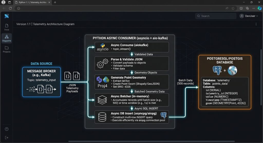
A common pitfall in streaming pipelines is inserting records into the database one event at a time over single synchronous database connections. This creates network latency bottlenecks and risks locking resources.
The Python consumer pipeline implementation below uses
confluent-kafka for non-blocking message fetching, standard spatial validation checks, psycopg2 connection pooling, and PostGIS execute_values batch inserts.Python
import json
import logging
from datetime import datetime, timezone
import psycopg2
from psycopg2 import pool
from psycopg2.extras import execute_values
from confluent_kafka import Consumer, KafkaError, KafkaException

logging.basicConfig(level=logging.INFO, format="%(asctime)s [%(levelname)s] %(message)s")

# Database Pool Configuration
DB_POOL = psycopg2.pool.ThreadedConnectionPool(
    minconn=2,
    maxconn=10,
    dbname="spatial_db",
    user="postgres",
    password="secure_password",
    host="localhost",
    port="5432"
)

# Kafka Consumer Configuration
KAFKA_CONFIG = {
    'bootstrap.servers': 'localhost:9092',
    'group.id': 'postgis-spatial-ingestion-group',
    'auto.offset.reset': 'earliest',
    'enable.auto.commit': False
}

BATCH_SIZE = 500  # Number of records per database transaction
POLL_TIMEOUT = 1.0  # Seconds

def validate_and_parse_payload(payload_str):
    """Parses JSON, validates spatial bounds, and formats geometry parameters."""
    try:
        data = json.loads(payload_str)
        lon = float(data['longitude'])
        lat = float(data['latitude'])
        alt = float(data.get('altitude_m', 0.0))

        # WGS84 Spatial Validation Boundary Check
        if not (-180.0 <= lon <= 180.0 and -90.0 <= lat <= 90.0):
            logging.warning(f"Invalid spatial coordinates: lon={lon}, lat={lat}")
            return None

        # Return structured parameter tuple matching SQL inputs
        return (
            data['vehicle_id'],
            data['timestamp'],
            lon, lat, alt, # Used in ST_SetSRID(ST_MakePoint(x, y, z), 4326)
            data.get('speed_kmh'),
            data.get('heading_deg'),
            data.get('accuracy_m')
        )
    except (KeyError, ValueError, TypeError) as err:
        logging.error(f"Payload validation failed: {err}")
        return None

def flush_batch_to_postgis(batch):
    """Executes bulk inserts into historical history and upserts current state."""
    if not batch:
        return True

    conn = DB_POOL.getconn()
    try:
        with conn.cursor() as cursor:
            # 1. Bulk Insert into Historical Track Partition
            insert_history_query = """
                INSERT INTO vehicle_telemetry_history
                (vehicle_id, recorded_at, geom, speed_kmh, heading_deg, accuracy_m)
                VALUES %s;
            """
            # Template converting raw X, Y, Z float values into PostGIS PointZ Geometry
            template = """(
                %s, %s,
                ST_SetSRID(ST_MakePoint(%s, %s, %s), 4326),
                %s, %s, %s
            )"""

            execute_values(cursor, insert_history_query, batch, template=template, page_size=len(batch))

            # 2. Bulk Upsert Current State Table
            upsert_state_query = """
                INSERT INTO vehicle_current_state (vehicle_id, last_updated, geom, speed_kmh, heading_deg)
                VALUES %s
                ON CONFLICT (vehicle_id) DO UPDATE SET
                    last_updated = EXCLUDED.last_updated,
                    geom = EXCLUDED.geom,
                    speed_kmh = EXCLUDED.speed_kmh,
                    heading_deg = EXCLUDED.heading_deg,
                    updated_at = CURRENT_TIMESTAMP
                WHERE EXCLUDED.last_updated > vehicle_current_state.last_updated;
            """
            state_template = """(
                %s, %s,
                ST_SetSRID(ST_MakePoint(%s, %s, %s), 4326),
                %s, %s
            )"""
            # Filter batch tuple columns for the state upsert statement
            state_batch = [(item[0], item[1], item[2], item[3], item[4], item[5], item[6]) for item in batch]
            execute_values(cursor, upsert_state_query, state_batch, template=state_template, page_size=len(state_batch))

        conn.commit()
        return True
    except Exception as db_err:
        conn.rollback()
        logging.error(f"Database batch commit failed: {db_err}")
        return False
    finally:
        DB_POOL.putconn(conn)

def main():
    consumer = Consumer(KAFKA_CONFIG)
    consumer.subscribe(['vehicle-telemetry-raw'])
    logging.info("Kafka Spatial Consumer initialized. Listening for data streams...")

    current_batch = []

    try:
        while True:
            msg = consumer.poll(timeout=POLL_TIMEOUT)

            if msg is None:
                if current_batch:
                    if flush_batch_to_postgis(current_batch):
                        consumer.commit(asynchronous=False)
                        current_batch.clear()
                continue

            if msg.error():
                if msg.error().code() == KafkaError._PARTITION_EOF:
                    continue
                else:
                    raise KafkaException(msg.error())

            record = validate_and_parse_payload(msg.value().decode('utf-8'))
            if record:
                current_batch.append(record)

            if len(current_batch) >= BATCH_SIZE:
                if flush_batch_to_postgis(current_batch):
                    consumer.commit(asynchronous=False)
                    current_batch.clear()

    except KeyboardInterrupt:
        logging.info("Terminating consumer execution process...")
    finally:
        consumer.close()
        DB_POOL.closeall()

if __name__ == '__main__':
    main()
Step 4: Optimizing Write Throughput and PostGIS Performance
When working with high-throughput streams, standard spatial database configurations can bottleneck write rates. Optimizing PostGIS performance requires tuning PostgreSQL memory allocations, write-ahead logging (WAL), and spatial function parameters.
                  ┌─────────────────────────────────┐
                  │    In-Memory Processing Engine  │
                  └────────────────┬────────────────┘
                                   │
                    Prepared Batch Tuple Execution
                                   │
                                   ▼
┌─────────────────────────────────────────────────────────────────────┐
│                    PostgreSQL Engine Execution                       │
│                                                                     │
│  ┌──────────────────────┐             ┌──────────────────────────┐  │
│  │ ST_MakePoint Construction │             │  WAL Sequence Buffer     │  │
│  └──────────┬───────────┘             └────────────┬─────────────┘  │
│             │                                      │                │
│             ▼                                      ▼                │
│  ┌──────────────────────┐             ┌──────────────────────────┐  │
│  │ GiST R-Tree Indexing │             │ Asynchronous Page Flushes│  │
│  └──────────────────────┘             └──────────────────────────┘  │
└─────────────────────────────────────────────────────────────────────┘
1. Spatial Geometry Assembly Optimization
Avoid invoking spatial parsing tools like
ST_GeomFromText() or ST_GeomFromGeoJSON() inside stream-ingestion SQL loops. Parsing string abstractions like WKT (Well-Known Text) introduces avoidable CPU overhead.Instead, construct points natively using
ST_SetSRID(ST_MakePoint(longitude, latitude, elevation), 4326). For extreme throughput cases, convert binary positions into standard Extended Well-Known Binary (EWKB) format within Python prior to passing raw byte arrays directly to PostGIS.2. Tuning Database Parameters (postgresql.conf)
Adjust parameters in
postgresql.conf to handle streaming write loads:Ini, TOML
# Memory Configuration
shared_buffers = 4GB                  # 25% of total dedicated RAM
work_mem = 64MB                       # Memory allocated for internal sort operations
maintenance_work_mem = 512MB          # Accelerates spatial index generation

# Write-Ahead Log (WAL) Optimization for High Write Rates
wal_level = minimal
synchronous_commit = off              # Disables sync wait per commit for low-latency writes
checkpoint_completion_target = 0.9    # Smooths out I/O spikes during checkpoints
max_wal_size = 16GB
min_wal_size = 2GB

# Parallel Query Capabilities
max_worker_processes = 8
max_parallel_workers_per_gather = 4
Caution: Settingsynchronous_commit = offprovides significant write performance gains by decoupling physical disk writes from transaction completion responses. However, in the event of an ungraceful server power disruption, the last few milliseconds of committed stream transactions could be lost.
3. Connection Pooling Architecture
Direct database connection creations carry significant execution costs. Every connection involves process allocation, memory configuration, and credential authentication.
Using external connection pools such as PgBouncer in transaction mode—or using internal threaded pools (as demonstrated above with
psycopg2.pool)—keeps connection pools warm. This minimizes backend thread contention and ensures consistent streaming throughput.Step 5: Kafka Connect PostGIS Sink (Alternative No-Code Architecture)
If maintaining custom Python execution engines adds unwanted operational complexity, consider using standard Kafka Connect frameworks. You can use the JDBC Sink Connector or specialized Kafka Debezium modules to stream telemetry directly from Kafka topics into PostGIS tables without custom application code.
Kafka Connect Sink JSON Configuration
Save the following configuration as
postgis-sink-connector.json and post it to your Kafka Connect distributed REST API:JSON
{
  "name": "postgis-spatial-sink-connector",
  "config": {
    "connector.class": "io.confluent.connect.jdbc.JdbcSinkConnector",
    "tasks.max": "4",
    "topics": "vehicle-telemetry-raw",
    "connection.url": "jdbc:postgresql://localhost:5432/spatial_db",
    "connection.user": "postgres",
    "connection.password": "secure_password",
    "insert.mode": "upsert",
    "pk.mode": "record_key",
    "pk.fields": "vehicle_id",
    "table.name.format": "vehicle_current_state",
    "auto.create": "false",
    "auto.evolve": "false",
    "batch.size": "1000",
    "transforms": "addValidSpatialGeom",
    "transforms.addValidSpatialGeom.type": "org.apache.kafka.connect.transforms.InsertField$Value",
    "transforms.addValidSpatialGeom.static.field": "srid",
    "transforms.addValidSpatialGeom.static.value": "4326"
  }
}
Step 6: Real-Time Spatial Queries & Downstream Visualization
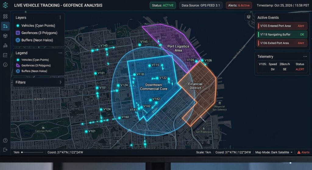
With your spatio-temporal telemetry stream continually updating PostGIS, you can execute real-time spatial calculations and power dynamic web dashboards.
1. Dynamic Geofencing Violations
Identify active vehicles operating outside a designated safe operational geofence zone:
SQL
SELECT
    v.vehicle_id,
    v.last_updated,
    ST_AsText(v.geom) AS current_position,
    ST_Distance(v.geom::geography, g.fence_geom::geography) AS meters_outside_geofence
FROM vehicle_current_state v
CROSS JOIN geofence_zones g
WHERE g.zone_name = 'Nairobi Central Sector'
  AND NOT ST_Within(v.geom, g.fence_geom);
2. Spatio-Temporal Windowing Analysis
Calculate rolling distance and average operational speeds using PostgreSQL window functions:
SQL
SELECT
    vehicle_id,
    recorded_at,
    speed_kmh,
    ST_Distance(
        geom::geography,
        LAG(geom, 1) OVER (PARTITION BY vehicle_id ORDER BY recorded_at)::geography
    ) AS step_distance_meters
FROM vehicle_telemetry_history
WHERE recorded_at >= NOW() - INTERVAL '1 hour'
  AND vehicle_id = 'v-8942-kenya'
ORDER BY recorded_at DESC;
3. Consuming Live Layers in QGIS and Web Dashboards
Once data is stored in standard PostGIS layers, real-time spatial web applications can query spatial features through GeoServer, MapServer, or custom FastAPI routes.
For desktop analysis, connect your PostGIS database directly to QGIS to configure real-time rendering layers that auto-refresh on defined intervals.
Conclusion
Managing spatio-temporal data streams requires an architecture that can isolate high-speed ingestion from spatial query workloads. By placing Apache Kafka at the front of your pipeline, you create a scalable, decoupled message layer capable of handling fluctuating IoT traffic. Paired with a optimized Python consumer layer and PostGIS, this architecture delivers low-latency ingestion alongside high-performance spatial analytics.
Whether building connected vehicle platforms, dynamic delivery dispatch networks, or smart-city monitoring infrastructure, this decoupled streaming stack provides a foundation that scales with your data requirements.