
Spatial Multi-Criteria Decision Analysis (MCDA) in Python: Automating Weighted Linear Combinations
Introduction
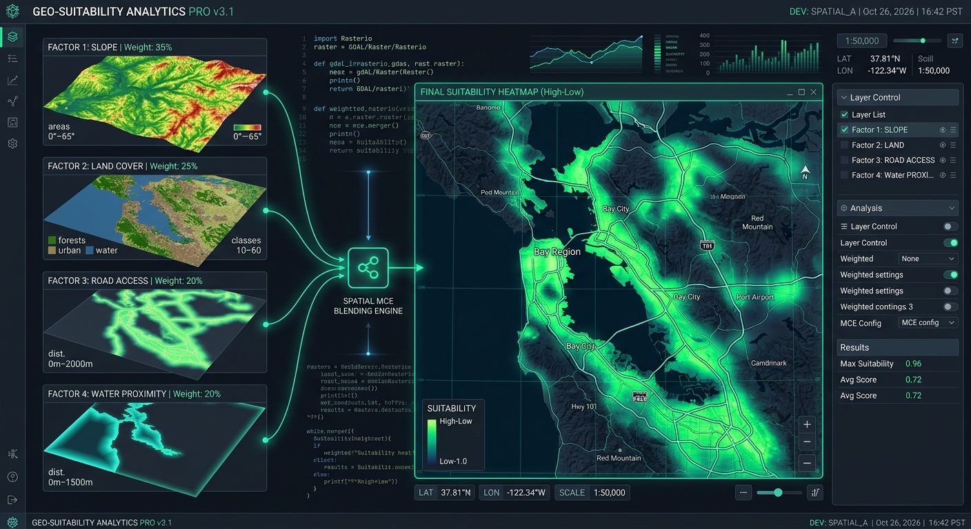
“When applying Spatial MCDA Python Weighted Linear Combinations workflows, geospatial analysts often need to automate multi-factor suitability evaluations efficiently. Selecting the best locations for solar farms, hospitals, conservation areas, or infrastructure projects often requires evaluating multiple geographic factors simultaneously. A site may have favorable terrain but poor road access, suitable land cover but unstable soil, or good accessibility while overlapping a protected ecosystem.
Geographic Information Systems (GIS) solve this problem through Multi-Criteria Decision Analysis (MCDA), which combines spatial criteria into a suitability surface. However, repeatedly adjusting weights and recalculating raster overlays in desktop GIS software becomes inefficient when researchers need to compare hundreds of scenarios, document decisions, or integrate suitability modeling into automated workflows.
Spatial MCDA in Python using Weighted Linear Combination (WLC) provides a reproducible alternative. With Rasterio and NumPy, analysts can standardize input rasters, calculate weighted suitability scores, apply exclusion constraints, and export continuous suitability maps without manually operating a raster calculator.
Weighted Linear Combination assigns each criterion a weight representing its relative importance. Standardized criterion values are multiplied by their weights and added together to produce a suitability score. Boolean masks then exclude areas that violate essential requirements.
This guide develops an automated Python workflow for evaluating potential solar farm locations. It covers raster alignment, fuzzy membership transformations, weight configuration, exclusion constraints, GeoTIFF export, and sensitivity analysis.
1. Understanding Spatial MCDA and Weighted Linear Combination
A typical GIS suitability model combines two types of information:
- Factors: Variables that influence how suitable a location is, such as slope, distance to roads, land cover, and soil stability.
- Constraints: Conditions that make locations unacceptable, such as protected areas, wetlands, or legally restricted land.
Because these criteria use different units, they must first be standardized to a common scale. A slope raster measured in degrees cannot be meaningfully added directly to a road-distance raster measured in meters.
Weighted Linear Combination addresses this problem by using standardized criterion scores ranging from 0 to 1.
The basic formula is:
[
S = \sum_{i=1}^{n} w_i x_i
]
Where:
- (S) is the final suitability score.
- (w_i) is the weight assigned to criterion (i).
- (x_i) is the standardized suitability value of criterion (i).
- (n) is the number of criteria.
Weights should be nonnegative and sum to one:
[
\sum_{i=1}^{n} w_i = 1
]
To incorporate exclusion constraints, extend the expression to:
[
S_c = \left(\sum_{i=1}^{n} w_i x_i\right)
\prod_{j=1}^{m} c_j
]
Here, each (c_j) is a binary constraint: 1 for an allowed location and 0 for an excluded location.
In a raster implementation, it is usually better to represent excluded pixels as NoData in the final suitability raster rather than assigning them an ordinary suitability score of zero. This preserves the distinction between an unsuitable location and a location that is prohibited or outside the analysis area.
2. Environment Setup and Input Data
Install the required Python packages in your project environment:
pip install rasterio numpy matplotlibRasterio handles raster reading, reprojection, and GeoTIFF writing. NumPy performs array calculations, while Matplotlib provides visualization.
Rasterio’s official documentation explains how datasets retain geospatial metadata during reading and writing, while its reprojection documentation describes how to transform source rasters to a destination grid. Rasterio Quickstart · Rasterio Reprojection.
Example input layers for solar farm suitability
| Raster | Example values | Role |
|---|---|---|
slope_deg.tif |
Slope in degrees | Favor flatter terrain |
landcover.tif |
Integer land-cover codes | Prefer suitable land-cover categories |
road_distance.tif |
Distance in meters | Favor accessible locations |
soil_stability.tif |
Stability index, 0–100 | Favor more stable soil |
protected_areas.tif |
0 = unrestricted, 1 = protected | Exclude restricted areas |
wetlands.tif |
0 = not wetland, 1 = wetland | Exclude wetlands |
The raster values and land-cover codes in this example are illustrative. Replace them with the classifications, engineering requirements, environmental regulations, and suitability thresholds appropriate for your study area.
For meaningful distance calculations, use an appropriate projected coordinate reference system (CRS) with linear units, such as meters. A raster using geographic coordinates in degrees should not be treated as though its pixel dimensions were meters.
3. Align All Rasters to a Common Grid
Before performing a raster overlay, every input must share the same:
- Coordinate reference system.
- Spatial resolution.
- Grid origin and affine transform.
- Width, height, and geographic extent.
Matching array dimensions alone does not guarantee spatial alignment. Two rasters can have identical shapes but represent different geographic locations.
Use one raster as the reference grid. In this example, the slope raster defines the output grid.
Read and align raster data
import rasterio
import numpy as np

from rasterio.warp import reproject
from rasterio.enums import Resampling


def read_aligned(path, reference, resampling):
    """Read a raster and align it to the reference grid."""

    with rasterio.open(path) as src:
        if src.crs is None or reference.crs is None:
            raise ValueError(
                f"Missing CRS in {path} or reference raster."
            )

        # Convert masked cells to NaN.
        source = src.read(1, masked=True)
        source = source.astype(np.float32).filled(np.nan)

        destination = np.full(
            (reference.height, reference.width),
            np.nan,
            dtype=np.float32
        )

        reproject(
            source=source,
            destination=destination,
            src_transform=src.transform,
            src_crs=src.crs,
            src_nodata=np.nan,
            dst_transform=reference.transform,
            dst_crs=reference.crs,
            dst_nodata=np.nan,
            resampling=resampling
        )

    return destination
The function reprojects each source to the reference raster’s CRS, transform, and dimensions. Invalid source cells are represented by NaN, allowing them to be excluded from subsequent calculations.
Choose the resampling method according to the data type:
- Bilinear: Suitable for continuous variables such as slope, road distance, and soil stability.
- Nearest neighbor: Suitable for categorical land-cover codes and binary exclusion masks.
Nearest-neighbor resampling preserves the original categories. Bilinear interpolation is useful for continuous surfaces because it estimates values from neighboring cells, although it can smooth local variation. See the Rasterio resampling documentation.
A multi-band GeoTIFF can also be read directly into a NumPy array:
with rasterio.open("criteria_stack.tif") as src:
    stack = src.read()

print(stack.shape)  # (bands, rows, columns)
A band stack is convenient when its bands are already aligned and have known meanings. Rasters stored in separate files still need to be aligned before combining their arrays.
4. Load the Suitability Criteria
With the helper function defined, load the four decision factors and two exclusion layers.
with rasterio.open("slope_deg.tif") as reference:
    profile = reference.profile.copy()

    slope = read_aligned(
        "slope_deg.tif", reference,
        Resampling.bilinear
    )

    landcover = read_aligned(
        "landcover.tif", reference,
        Resampling.nearest
    )

    road_distance = read_aligned(
        "road_distance.tif", reference,
        Resampling.bilinear
    )

    soil_stability = read_aligned(
        "soil_stability.tif", reference,
        Resampling.bilinear
    )

    protected = read_aligned(
        "protected_areas.tif", reference,
        Resampling.nearest
    )

    wetlands = read_aligned(
        "wetlands.tif", reference,
        Resampling.nearest
    )
Each returned array has the same row and column dimensions as the reference raster. The values now correspond to the same ground locations, making pixel-by-pixel calculations meaningful.
For especially large rasters, consider windowed reading and writing rather than loading every layer into memory at once.
5. Normalize Criteria Using Fuzzy Membership Functions
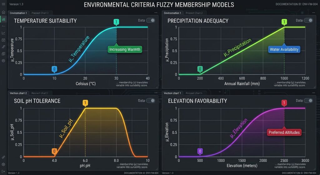
Normalization converts raw measurements into standardized suitability values between 0 and 1.
A score of 1 represents the most desirable value under the chosen model, while 0 represents the least desirable value. Intermediate scores represent intermediate suitability.
The direction of the transformation depends on the criterion. A solar farm may favor lower slopes but greater soil stability.
Linear decreasing membership
Use a decreasing transformation when lower raw values are more desirable:
[
\mu_{\downarrow}(x)=
\operatorname{clip}
\left(
\frac{x_{\max}-x}{x_{\max}-x_{\min}},
0,1
\right)
]
For example, define slope as fully suitable at or below 0 degrees and progressively less suitable until 15 degrees.
def linear_decreasing(values, best, worst):
    """Higher suitability for lower raw values."""
    if worst <= best:
        raise ValueError("'worst' must be greater than 'best'.")

    return np.clip(
        (worst - values) / (worst - best),
        0.0, 1.0
    )
Linear increasing membership
Use an increasing transformation when higher raw values are more desirable:
def linear_increasing(values, worst, best):
    """Higher suitability for higher raw values."""
    if best <= worst:
        raise ValueError("'best' must be greater than 'worst'.")

    return np.clip(
        (values - worst) / (best - worst),
        0.0, 1.0
    )
These functions apply explicit, interpretable thresholds. For instance, soil stability can receive zero suitability at an index of 0 and full suitability at 100.
Thresholds should come from domain knowledge, engineering requirements, empirical evidence, or stakeholder agreements. Avoid choosing thresholds solely because they produce an attractive map.
Normalize slope, road distance, and soil stability
slope_score = linear_decreasing(
    slope, best=0, worst=15
)

road_score = linear_decreasing(
    road_distance, best=0, worst=3000
)

stability_score = linear_increasing(
    soil_stability, worst=0, best=100
)
Under these assumptions, flat terrain receives the highest slope score, locations closer to roads receive greater accessibility scores, and soil with a stability index near 100 receives the highest stability score.
A separate constraint will exclude sites too close to roads if the project’s setback rules require it.
Convert categorical land cover to suitability
Categorical values should not automatically be processed with a continuous linear function. A land-cover code of 4 is not necessarily twice as suitable as a code of 2.
Instead, assign each category a score based on project objectives.
landcover_score = np.full(
    landcover.shape,
    np.nan,
    dtype=np.float32
)

# Illustrative land-cover codes:
# 1 = barren land
# 2 = grassland or shrubland
# 3 = cropland
# 4 = forest
# 5 = wetland or water

landcover_scores = {
    1: 1.0,
    2: 0.8,
    3: 0.5,
    4: 0.0,
    5: 0.0
}

for code, score in landcover_scores.items():
    landcover_score[landcover == code] = score
Unknown categories remain NaN instead of silently receiving an arbitrary suitability score. Adjust this lookup table to match the actual coding scheme and land-use policy for your study area.
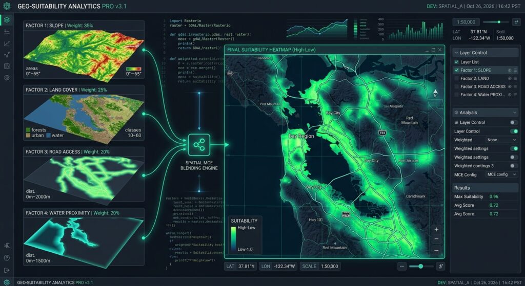
Image 1 placeholder: Multi-layer input raster stack combining into a single suitability output map
Alt text: Diagram showing individual spatial factor maps (slope, land use, road distance) stacking together into a single color-coded site suitability raster map.
6. Calculate the Weighted Linear Combination
Once all criteria have been standardized, define their relative importance.
For this solar farm example, use:
| Criterion | Weight |
|---|---|
| Slope | 0.35 |
| Land cover | 0.30 |
| Road accessibility | 0.20 |
| Soil stability | 0.15 |
| Total | 1.00 |
These are demonstration weights, not universal recommendations. An actual project should establish weights through expert judgment, stakeholder consultation, an Analytical Hierarchy Process (AHP), or another defensible decision-making method.
Check that the weights sum to one before calculating the suitability surface.
weights = {
    "slope": 0.35,
    "landcover": 0.30,
    "road": 0.20,
    "stability": 0.15
}

if not np.isclose(sum(weights.values()), 1.0):
    raise ValueError("Criterion weights must sum to 1.")
Now calculate the suitability score:
criteria = np.stack([
    slope_score,
    landcover_score,
    road_score,
    stability_score
])

weight_array = np.array([
    weights["slope"],
    weights["landcover"],
    weights["road"],
    weights["stability"]
], dtype=np.float32)

# Keep only cells with valid values in every criterion.
valid = np.all(np.isfinite(criteria), axis=0)

suitability = np.full(
    slope.shape,
    np.nan,
    dtype=np.float32
)

weighted_score = np.tensordot(
    weight_array,
    np.nan_to_num(criteria, nan=0.0),
    axes=(0, 0)
)

suitability[valid] = weighted_score[valid]
The result is a continuous suitability surface with values between 0 and 1. Larger values indicate locations that perform better under the model’s chosen criteria and weights.
This is a compensatory model: a high score on one criterion can offset a low score on another. That is why hard constraints must be handled separately.
7. Apply Boolean Exclusion Constraints
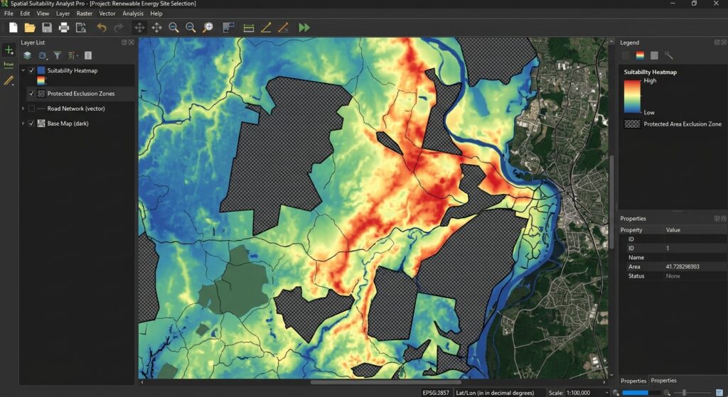
Some requirements are non-negotiable. A location inside a legally protected area should not become acceptable simply because it has good road access and flat terrain.
For this example, exclude:
- Protected areas.
- Wetlands and water bodies where development is prohibited.
- Slopes steeper than 20 degrees.
- Locations within a 50-meter road setback.
These are illustrative project rules and should be replaced with applicable environmental and planning requirements.
known_constraints = (
    np.isfinite(slope)
    & np.isfinite(protected)
    & np.isfinite(wetlands)
    & np.isfinite(road_distance)
)

allowed = (
    known_constraints
    & (slope <= 20)
    & (protected == 0)
    & (wetlands == 0)
    & (road_distance >= 50)
)

constrained_suitability = np.where(
    allowed & valid,
    suitability,
    np.nan
)
This implementation combines the weighted suitability score with Boolean eligibility rules. Areas that violate any of the constraints are marked as NaN.
Notice that the fuzzy slope membership reaches zero at 15 degrees, whereas the hard exclusion begins above 20 degrees. This distinction is intentional: a location can be technically eligible yet have a low suitability score.
Image 2 placeholder: Continuous suitability heatmap comparison (Unconstrained vs Constrained)
Alt text: GIS suitability heatmap illustrating high-suitability green zones versus red excluded zones masked by environmental constraints.
8. Export the Suitability Surface to GeoTIFF
The final step is to save the continuous suitability surface while retaining the reference raster’s spatial metadata.
Use a defined NoData value for excluded or invalid pixels when writing the file.
output_nodata = -9999.0

output_array = np.where(
    np.isfinite(constrained_suitability),
    constrained_suitability,
    output_nodata
).astype(np.float32)

profile.update(
    driver="GTiff",
    count=1,
    dtype="float32",
    nodata=output_nodata,
    compress="deflate"
)

with rasterio.open(
    "solar_farm_suitability.tif",
    "w",
    **profile
) as dst:
    dst.write(output_array, 1)

print("Saved solar_farm_suitability.tif")
The resulting GeoTIFF contains a single floating-point band, a compatible CRS and grid transform, and a declared NoData value. It can be opened in QGIS or another GIS application for visualization and further analysis.
For a quick preview, plot the output:
import matplotlib.pyplot as plt

display_data = np.ma.masked_equal(
    output_array,
    output_nodata
)

plt.figure(figsize=(10, 7))
plt.imshow(display_data, cmap="RdYlGn", vmin=0, vmax=1)
plt.colorbar(label="Suitability (0–1)")
plt.title("Solar Farm Site Suitability")
plt.axis("off")
plt.tight_layout()
plt.show()
This color ramp displays higher scores in green and lower scores in red. Excluded pixels are masked from the plot; configure their appearance separately in QGIS if you want to display them in a distinct color.
9. Automate Weight Scenarios and Sensitivity Analysis
One of the strongest reasons to automate spatial MCDA is the ability to test alternative decision assumptions.
For example, a solar developer may prioritize road accessibility, while an environmental planning team may emphasize land cover and slope. Rather than manually rebuilding each raster overlay, evaluate several weight configurations using the same normalized criteria.
scenarios = {
    "balanced": [0.35, 0.30, 0.20, 0.15],
    "access_priority": [0.25, 0.25, 0.35, 0.15],
    "environment_priority": [0.40, 0.40, 0.10, 0.10]
}

for name, scenario_weights in scenarios.items():
    w = np.asarray(
        scenario_weights,
        dtype=np.float32
    )

    if not np.isclose(w.sum(), 1.0):
        raise ValueError(
            f"Weights for {name} do not sum to 1."
        )

    score = np.tensordot(
        w,
        np.nan_to_num(criteria, nan=0.0),
        axes=(0, 0)
    )

    score[~valid] = np.nan
    score[~allowed] = np.nan

    print(
        name,
        "mean eligible suitability:",
        float(np.nanmean(score))
    )
The values are illustrative scenarios. For more extensive analysis, generate hundreds of weight combinations, preserve their outputs, and compare changes in top-ranked locations or the proportion of eligible land in the highest suitability class.
When interpreting results, remember that weights are only one source of uncertainty. Raster resolution, input data quality, normalization thresholds, classification decisions, and constraints can also change rankings.
Using AHP to derive weights
The Analytical Hierarchy Process (AHP) is a structured method for converting pairwise comparisons into criterion weights. Decision-makers compare the importance of two criteria at a time, producing a comparison matrix from which normalized weights can be calculated.
Those weights can then be passed to the WLC function above. In practical projects, inspect AHP consistency and document who supplied the judgments and why. A normalized set of weights does not automatically mean those judgments are valid or unbiased.
10. Practical Limitations and Best Practices
Keep normalization consistent. When comparing study areas or scenarios, use the same criterion thresholds. Calculating a new minimum and maximum for every region can make suitability scores incomparable.
Validate input data. Confirm that raster values, units, CRS definitions, and categorical codes are correct. An incorrectly interpreted land-cover code can invalidate the final model even if the NumPy calculations are perfect.
Preserve NoData semantics. Distinguish missing information from genuinely low suitability. If a required criterion has no valid data for a pixel, do not silently treat that absence as a score of zero.
Consider model sensitivity. Review how changes to weights and fuzzy thresholds affect the highest-ranked locations. Areas that remain highly suitable across many scenarios are often more robust candidates for further investigation.
Account for computational scale. The example loads complete rasters into memory. For very large study areas, process aligned rasters in matching windows or blocks and write results incrementally. Every window must use the same grid alignment, and calculations must apply identical weights, transformations, and constraints.
Do not treat suitability as a final decision. A high MCDA score indicates relative suitability under the chosen assumptions. It does not replace field surveys, land ownership checks, engineering assessments, biodiversity assessments, or regulatory approval.
11. SEO Interlinking and Further Reading
Build topical authority by linking this article to related geospatial automation tutorials.
Suggested internal links:
- Analytical Hierarchy Process (AHP) Decision Analysis — explain how expert judgments can be converted into criterion weights.
- QGIS Raster Calculator Tutorial — compare manual raster overlays with automated Python workflows.
- GeoTIFF Processing with Python — cover raster metadata, reprojection, and export.
Replace these suggested paths with the corresponding live URLs on your site.
Recommended external references:
- Rasterio Documentation — raster reading, reprojection, resampling, and output writing.
- NumPy Documentation — array arithmetic, masking, stacking, and numerical transformations.
- Rasterio Resampling Guide — choosing suitable resampling methods for different raster types.
- Rasterio Reprojection Guide — matching rasters to a common spatial grid.
Conclusion
Spatial MCDA in Python makes suitability modeling reproducible, scalable, and easier to audit. By combining Rasterio for geospatial raster handling with NumPy for normalization, weighted overlays, and Boolean masks, GIS analysts can automate multi-factor site selection without repeatedly rebuilding desktop raster calculator expressions.
The workflow developed here standardizes terrain, land-cover, accessibility, and soil-stability criteria; combines them using Weighted Linear Combination; excludes restricted locations; and exports the final continuous suitability surface as a GeoTIFF.
For real-world deployment, the most important considerations are defensible normalization thresholds, appropriate criterion weights, strict raster alignment, explicit treatment of NoData, and sensitivity analysis. Together, these practices turn a simple raster overlay into a more transparent spatial decision-support workflow that can be reused across projects and tested against alternative planning scenarios.