
Hyperspectral vs Multispectral Remote Sensing: Spectral Resolution Explained
1. Introduction: Why spectral resolution matters
Remote sensing allows researchers to investigate Earth’s surface by measuring electromagnetic energy reflected, emitted, or scattered by objects. Different materials interact with electromagnetic radiation differently, producing patterns that can help distinguish vegetation, soil, minerals, water, and built surfaces.
However, the usefulness of an image depends not only on the size of its pixels. It also depends on which wavelengths the sensor measures, how frequently observations are collected, and how accurately the instrument records differences in energy.
These characteristics are described by four fundamental dimensions of remote sensing: spatial, spectral, temporal, and radiometric resolution.
1.1 The four dimensions of remote sensing resolution
Spatial resolution — How much detail can the sensor distinguish?
A 10 m image pixel represents a smaller ground area than a 30 m pixel. Spatial resolution influences whether narrow roads, small fields, or individual objects can be distinguished.
Spectral resolution — How finely can the sensor distinguish wavelengths?
A sensor with many narrow spectral bands can capture subtle absorption features that may be averaged together in a broader band. This is central to distinguishing materials with similar overall reflectance.
Temporal resolution — How frequently can the area be observed?
Frequent observations help track crop growth, seasonal vegetation changes, flooding, and other processes that evolve over time.
Radiometric resolution — How finely can energy differences be recorded?
Radiometric resolution describes the sensor’s ability to represent differences in signal intensity. Higher bit depth allows more digital values, although actual sensitivity also depends on noise and instrument performance.
These dimensions are related, but they are not interchangeable. A sensor can have excellent spatial resolution and relatively limited spectral detail, or many spectral bands but comparatively coarse spatial resolution.
The fundamental distinction between multispectral and hyperspectral remote sensing is the amount and arrangement of spectral information collected for each ground pixel.
1.2 What is spectral resolution?
Spectral resolution describes how finely a sensor can distinguish wavelengths within the electromagnetic spectrum. It depends on the width and resolving capability of the sensor’s spectral channels.
A useful approximation for the bandwidth of an individual spectral band is:
where \(\lambda\) represents wavelength, commonly measured in nanometres (nm) for visible, near-infrared, and shortwave-infrared imagery.
For example, one sensor might measure energy across a band spanning 650–680 nm, while another records a narrower band spanning 660–670 nm. The narrower band captures a more restricted wavelength interval and may reveal a feature that the broader band averages out.
The number of bands alone does not completely determine spectral resolution. Bandwidth, spectral sampling intervals, response-function overlap, and signal-to-noise ratio also matter.
This brings us to the main comparison: multispectral sensors collect information in selected wavelength bands, while hyperspectral imaging systems measure many closely spaced, usually contiguous bands to reconstruct detailed spectral signatures.
2. Multispectral remote sensing: Selected bands for broad applications
2.1 Definition and operating principle
Multispectral remote sensing collects image data in a relatively small number of selected spectral bands. These bands are designed to capture useful portions of the electromagnetic spectrum rather than measure every narrow interval continuously.
Common multispectral systems include:
-
Landsat 8 and Landsat 9 — their Operational Land Imager (OLI) and Thermal Infrared Sensor (TIRS) provide visible, near-infrared, shortwave-infrared, and thermal observations. OLI has nine bands, including its panchromatic band, while TIRS adds two thermal bands.
-
Sentinel-2 — its Multispectral Instrument collects data in 13 bands, with spatial resolutions of 10, 20, or 60 metres depending on the band.
A multispectral sensor’s band selection reflects a scientific or operational purpose. Visible bands support color and surface characterization; near-infrared bands help distinguish vegetation from many non-vegetated surfaces; and shortwave-infrared bands respond to properties associated with vegetation moisture, soil conditions, and mineral composition.
For example, Sentinel-2 includes red-edge bands designed to capture changes in vegetation reflectance that are useful for studying vegetation condition.
2.2 How multispectral bands work
Consider a typical multispectral image with blue, green, red, near-infrared, and shortwave-infrared bands.
Each band records a value representing the energy received within its spectral response range. The values from different bands can be combined into color composites, indices, or classification features.
A common vegetation index is the Normalized Difference Vegetation Index (NDVI):
Healthy green vegetation typically reflects strongly in the near-infrared and absorbs much of the red light used for photosynthesis. NDVI exploits this contrast to characterize vegetation greenness and relative vigor.
Other multispectral applications include water-body delineation, burn severity assessment, urban land-cover mapping, crop classification, and cloud or snow detection. Carefully selected bands may distinguish many relevant land-cover classes without requiring hundreds of spectral measurements.
2.3 Strengths of multispectral imagery
Operational efficiency. Multispectral datasets are generally easier to store, process, and analyze than comparable hyperspectral datasets with the same spatial dimensions.
Broad geographic coverage. Missions such as Landsat and Sentinel-2 support repeat observations across large areas and have established data archives. This makes them useful for regional mapping and long-term change analysis.
Mature analytical methods. Common techniques such as NDVI, the Normalized Difference Water Index, supervised classification, and random-forest land-cover mapping are well supported by standard remote sensing and GIS software.
Frequent observation opportunities. The Sentinel-2 constellation, for example, offers a nominal five-day revisit at the equator under its standard mission configuration. That makes it useful for regular agricultural and environmental monitoring, subject to cloud cover and actual acquisition availability.
2.4 Limitations: When broad bands are not enough
Multispectral imagery can struggle to differentiate materials whose reflectance patterns are similar over the selected bands.
Imagine two minerals that have similar reflectance in blue, green, red, and near-infrared wavelengths, but differ in the exact position and shape of an absorption feature in the shortwave-infrared region. If the feature falls within a broad band, its signature may be averaged together with the surrounding reflectance.
The same challenge occurs in vegetation studies. Several tree species can appear spectrally similar in a handful of broad bands, particularly if they have comparable canopy structure, moisture content, and phenological stage.
Multispectral imagery may still distinguish those species when combined with seasonal observations, texture, topography, or other environmental variables. The limitation is not that multispectral data can never distinguish similar materials; it is that the sensor may not capture enough spectral detail to separate them reliably on spectral evidence alone.
Best suited to: regional land-cover classification, vegetation indices, crop monitoring, flood mapping, burn assessment, and repeatable environmental monitoring.
3. Hyperspectral remote sensing: Detailed spectral signatures
3.1 Definition and operating principle
Hyperspectral remote sensing, also called imaging spectroscopy, collects measurements in hundreds of narrow, closely spaced spectral channels. These channels generally form a contiguous spectrum across a specified wavelength range.
Examples include:
-
AVIRIS — an airborne imaging spectrometer with 224 contiguous spectral channels covering approximately 400–2500 nm in its classic configuration.
-
EnMAP — a spaceborne imaging spectroscopy mission whose data cover the visible and near-infrared through shortwave-infrared regions, with 224 contiguous bands reported for the operational spectral data. Its ground sampling distance is approximately 30 metres.
-
PRISMA — an imaging spectroscopy satellite providing 240 spectral bands across its visible/near-infrared and shortwave-infrared channels, alongside a separate panchromatic camera.
Instead of measuring only a handful of broad wavelength intervals, a hyperspectral sensor records a more detailed reflectance or radiance profile for each pixel.
The output is commonly represented as a hyperspectral data cube:
-
Two dimensions describe the spatial arrangement of pixels.
-
The third dimension contains measurements across wavelength.
Each pixel therefore has an associated spectrum rather than only a few independent band values.
3.2 Narrow contiguous bands versus broad bands
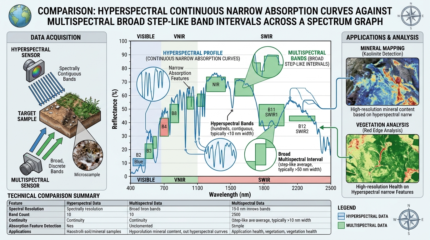
The difference is easiest to understand by considering a hypothetical material with a narrow absorption feature.
Multispectral measurement
A few selected bands summarize reflectance over wider wavelength intervals.
Broad-band measurements can average a narrow absorption feature with adjacent wavelengths.
Hyperspectral measurement
Many narrow channels describe the shape and position of the absorption feature in greater detail.
Narrow contiguous channels help resolve the feature’s depth, shape, and wavelength position.
Figure 1. Conceptual illustration only—not real measurements from a sensor or a particular material.
A hyperspectral instrument can reveal differences in spectral shape that are hidden by broad-band averaging. However, the feature must still be sufficiently strong relative to sensor noise, atmospheric effects, and the composition of the pixel.
3.3 Why continuous spectral signatures are valuable
Different materials interact with radiation because of their physical and chemical properties. Minerals, plants, soils, and water can exhibit distinctive patterns of absorption and reflectance.
For mineral mapping, absorption features may be associated with particular molecular bonds or mineral structures. A hyperspectral sensor can record the position and shape of these features, allowing the measured spectrum to be compared with laboratory or field reference spectra. This is one of the foundations of imaging spectroscopy for mapping surface mineral composition.
Researchers may analyze spectral signatures using methods such as:
-
Spectral angle mapping.
-
Spectral feature fitting and continuum removal.
-
Matched filtering.
-
Linear spectral mixture analysis.
-
Classification and regression models trained on reference spectra.
For example, a mineral-mapping workflow may compare image spectra with a reference library to identify areas whose absorption features are consistent with minerals such as white mica, chlorite, clay minerals, or gypsum. The reliability of the result depends on the wavelength coverage, calibration, atmospheric correction, spatial resolution, and the purity of the observed surface.
3.4 Strengths of hyperspectral imagery
Greater material discrimination. Closely spaced spectral bands can separate materials whose diagnostic features fall between, or are diluted within, multispectral band intervals.
Mineral identification and mapping. Hyperspectral imagery is especially useful when surface minerals have diagnostic absorption features within the sensor’s wavelength range.
Detailed vegetation characterization. Fine spectral measurements can help distinguish plant functional traits, species, stress responses, and biochemical properties when the spectral information and ground reference data support that level of interpretation.
Advanced water-quality analysis. Hyperspectral observations can help characterize optically active water constituents, including chlorophyll-a, colored dissolved organic matter, and suspended particles. More specific pollutant detection is possible only when the target has a detectable spectral signature and environmental interference is sufficiently controlled.
Research into subtle surface differences. Detailed spectra support material identification, spectral unmixing, and quantitative estimation that may be difficult with a limited set of broad bands.
3.5 Limitations of hyperspectral imagery
More bands do not automatically mean better results.
Hyperspectral datasets often require greater storage, processing power, preprocessing, calibration, and specialized analytical methods. Their narrower bands may collect fewer photons per band, creating a trade-off between spectral detail and signal-to-noise ratio.
Other challenges include:
-
Atmospheric absorption and scattering that distort the measured spectrum.
-
Mixed pixels containing multiple materials.
-
Cloud, shadow, or vegetation cover obscuring the target surface.
-
Similar spectral signatures among related materials.
-
Limited availability of suitable field measurements or reference spectra.
-
Processing complexity and the risk of overfitting in classification models.
The USGS has documented how residual atmospheric artifacts can affect mineral identification, especially where absorption features are weak or mineral abundance is low.
Hyperspectral imagery is therefore not a replacement for field validation, laboratory spectroscopy, or supporting geological, ecological, and chemical information.
Best suited to: detailed mineral and material mapping, selected vegetation-species or biochemical studies, advanced water-quality research, and applications requiring diagnostic spectral signatures.
4. Direct comparison matrix: Multispectral versus hyperspectral
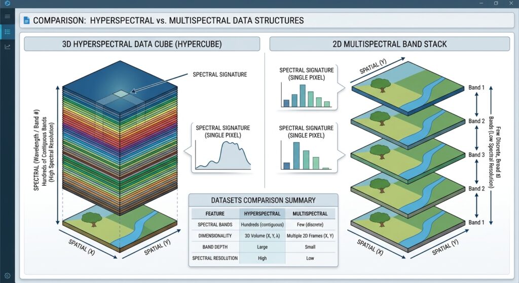
The most important distinction is not simply the number of bands. It is how much useful information those bands preserve about the shape of a material’s spectral signature.
| Comparison factor | Multispectral remote sensing | Hyperspectral remote sensing |
|---|---|---|
| Band count | Typically a handful to a few dozen selected bands | Commonly hundreds of narrow spectral channels |
| Band width | Usually broader, with widths varying by band and sensor | Usually narrow, closely spaced, and often contiguous |
| Spectral sampling | Selected portions of the spectrum | Dense sampling across a wavelength range |
| Data volume | Generally lower for equivalent image dimensions and bit depth | Generally higher because many more channels are stored |
| Feature discrimination | Effective for broad surface classes and many vegetation or water indicators | Better suited to subtle spectral differences and diagnostic absorption features |
| Common sensors | Landsat 8/9, Sentinel-2 | AVIRIS, EnMAP, PRISMA |
| Spatial resolution | Depends on sensor and band; Sentinel-2 includes 10, 20, and 60 m bands | Depends on sensor; EnMAP and PRISMA provide approximately 30 m hyperspectral imagery |
| Processing demands | Generally manageable using standard GIS workflows | Often requires more memory, calibration, atmospheric correction, and spectral analysis |
| Vegetation applications | NDVI, crop monitoring, land-cover classification | More detailed species, trait, pigment, and biochemical analysis when supported by data |
| Geological applications | Broad lithological discrimination and alteration screening | Detailed mineral mapping where diagnostic spectral features are measurable |
| Water applications | Water extent and selected water-quality proxies | More detailed analysis of optically active water constituents |
| Main limitation | Materials with similar responses in selected bands may remain difficult to separate | Noise, atmospheric effects, mixed pixels, data volume, and uncertain spectral references can limit identification |
The sensor specifications illustrate why these categories differ. Sentinel-2 acquires 13 spectral bands, AVIRIS Classic provides 224 contiguous channels, EnMAP provides 224 contiguous bands in its operational spectral data, and PRISMA provides 240 spectral bands. These are examples rather than universal thresholds separating the two technologies.
4.1 Why data volume increases
Suppose two image products cover the same ground area, contain the same number of pixels, and use the same number of bits per measurement.
A simplified estimate of uncompressed raster size is:
where:
-
\(V\) is the approximate storage size in bytes.
-
\(N_x\) and \(N_y\) are the raster dimensions.
-
\(N_b\) is the number of bands.
-
\(b\) is the number of bits stored per pixel per band.
For a hypothetical 1,000 × 1,000 image with 12-bit measurements stored in tightly packed form, 10 bands require approximately 15 MB, whereas 200 bands require approximately 300 MB.
In practical GeoTIFF products, measurements may be stored in 16-bit or 32-bit data types, and metadata, compression, masks, and processing intermediates also affect actual file size. Under equal storage assumptions, however, the 200-band dataset contains 20 times as many band values as the 10-band dataset.
This difference influences processing workflows. Large hyperspectral datasets may benefit from tiled storage, carefully chosen data types, dimensionality reduction, and analysis restricted to relevant wavelength ranges.
5. Practical research examples
Consider three research questions to see how the sensor choice changes with the scientific objective.
Case 1: Monitoring vegetation health across a county
Research objective: Identify declining vegetation and compare seasonal crop conditions across a large area.
A Sentinel-2 or Landsat workflow is usually a sound starting point. Calculate NDVI, use shortwave-infrared information where appropriate, mask cloud and shadow contamination, and analyze time series across the growing season.
Hyperspectral data may provide additional information about vegetation composition or traits, but it may not be necessary if the research question concerns broad greenness patterns and regional change.
Case 2: Identifying surface minerals around a potential mining area
Research objective: Distinguish alteration minerals and map their spatial distribution.
Hyperspectral imagery is generally preferable when the target minerals have diagnostic absorption features within the available spectral range.
A defensible workflow includes atmospheric correction, masking unreliable wavelengths and pixels, comparing the reflectance spectra with an appropriate spectral library, generating mineral maps, and validating the results using field samples or geological observations.
Multispectral data can still support regional geological screening, but broad spectral bands may not capture enough detail to discriminate closely related mineral species.
Case 3: Investigating water quality in a lake
Research objective: Estimate chlorophyll concentrations, suspended material, or changes in water optical properties.
Multispectral imagery can be effective for established water-quality indicators when the sensor has suitable bands and the retrieval model is calibrated for local conditions.
Hyperspectral imagery may offer an advantage where fine spectral features help separate optically active constituents. However, atmospheric correction over water, sunglint, water depth, turbidity, and mixed land-water pixels can complicate retrievals. Specific chemical pollutants should not be assumed detectable merely because hyperspectral data are available.
6. How to choose the right sensor for research
Use the following decision guide to identify which type of imagery better fits a project.
Research sensor selector
What is the main research objective?
What is the study scale?
What processing resources are available?
Recommended starting point
Multispectral imagery
Start with Sentinel-2 or Landsat for spectral indices, classification, and repeat monitoring. Use hyperspectral data if a clear additional research question requires finer spectral detail.
Regional coverage favors checking swath width, repeat acquisitions, cloud-free observations, and processing cost.Test the workflow on a representative study area and benchmark preprocessing and storage requirements before expanding.
Whatever sensor you select, assess the complete measurement design before beginning image analysis:
-
Spectral suitability: Do the bands cover the wavelengths that respond to the target material or process?
-
Spatial suitability: Is the target large enough to be represented reliably at the sensor’s ground sampling distance?
-
Temporal suitability: Do the acquisition dates capture the season or process being investigated?
-
Radiometric and atmospheric quality: Are the signals sufficiently reliable to resolve the expected differences?
-
Validation: Can the classifications or physical estimates be checked against field observations, laboratory measurements, or another independent reference?
These considerations often determine the quality of a research result more strongly than band count alone.
7. Conclusion: Hyperspectral vs Multispectral Remote Sensing Spectral Resolution Summary
Hyperspectral vs multispectral remote sensing is fundamentally a comparison of spectral information content and the scientific questions that information can answer.
Multispectral sensors collect measurements in selected bands and are effective for broad land-cover classification, vegetation indices, agricultural monitoring, and large-area environmental studies. Their established data archives and manageable processing requirements make them practical for many GIS applications.
Hyperspectral sensors record much denser spectral information, allowing researchers to examine the detailed shape and location of spectral features. This is particularly valuable for mineral identification, advanced vegetation analysis, and selected water-quality applications where diagnostic spectral information is available.
Nevertheless, hyperspectral imagery does not automatically deliver higher spatial resolution, more frequent observations, or reliable species-level identification. Its additional information is useful only when the target can be distinguished from noise, atmospheric interference, mixed pixels, and other confounding effects.
The guiding principle for research selection is to choose the sensor that resolves the scientific question—not simply the sensor with the most bands.
Further reading
-
NASA Earthdata — Remote Sensing Resolution: foundational concepts of spatial, spectral, temporal, and radiometric resolution.
-
ESA — Sentinel-2: multispectral instrument specifications and applications.
-
NASA/JPL — AVIRIS: airborne imaging spectroscopy and contiguous spectral channels.
-
DLR — EnMAP mission: hyperspectral observations, mission specifications, and research applications.
-
USGS — Spectroscopy Lab: spectral libraries and research on material identification and mineral mapping.