Querying OpenStreetMap Data at Scale with Python and DuckDB

1. Introduction: Why Combine OpenStreetMap with DuckDB?

To Query OpenStreetMap Data Python DuckDB effectively, regional extracts provide detailed, openly accessible geographic data covering roads, buildings, and amenities. OpenStreetMap (OSM) provides detailed, openly accessible geographic data covering roads, buildings, amenities, land use, and countless other geographic features. For large-scale GIS projects, however, obtaining the data is only the beginning.

Regional .osm.pbf files can contain millions of nodes, ways, and relations. Extracting every building in a country, selecting road classes across an entire region, or counting amenities by category can place substantial demands on memory and processing time when handled through traditional desktop GIS workflows.

A typical desktop workflow involves opening an OSM extract, converting it into usable geometry layers, applying filters, and exporting the resulting data. Repeating those operations for multiple study areas can be inefficient, particularly when the same source data supports dozens of different analyses.

Python and DuckDB offer a more flexible approach.

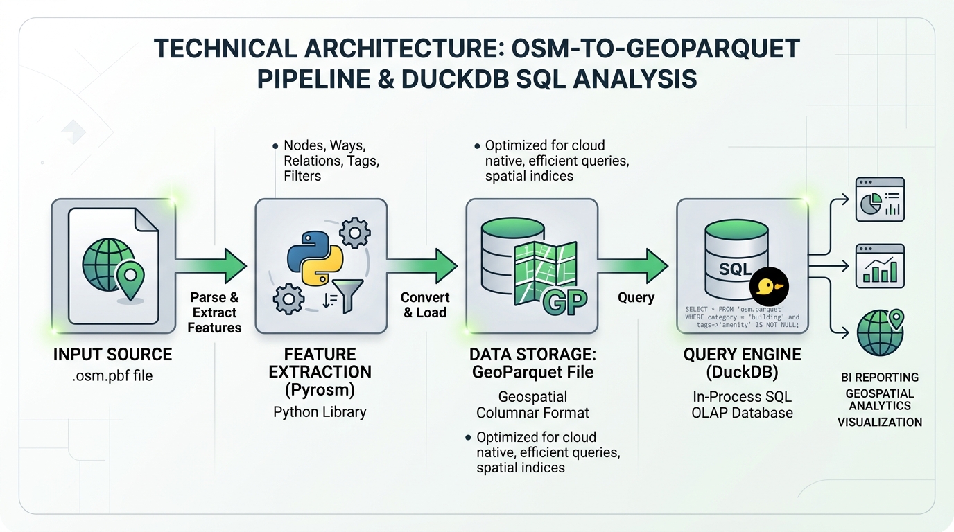
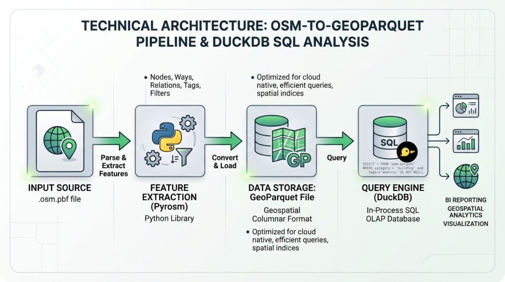
• Python and Pyrosm parse OSM PBF files into meaningful geographic feature layers, including roads, building footprints, and points of interest.
• DuckDB executes SQL queries locally, using columnar processing, parallel execution, and spatial functions to filter, aggregate, transform, and export large datasets.
• GeoParquet provides a reusable, compressed format for subsequent queries without repeatedly parsing the original PBF file.

DuckDB also has a native ST_ReadOSM() table function that reads compressed OSM PBF files directly. It uses multithreaded parsing, but returns raw OSM elements rather than automatically constructing building polygons or road geometries. For complete geometric layers, a PBF extraction tool such as Pyrosm is often the more straightforward solution.

The central principle: use an OSM-aware parser for feature reconstruction where necessary, then use DuckDB for repeated analytical queries over the resulting spatial data.

This distinction matters for performance. Filtering a prepared GeoParquet dataset may be very fast, but parsing a multi-gigabyte PBF and reconstructing its geometries can still take minutes or longer, depending on the data, hardware, and extraction requirements.

2. Setup and Prerequisites

2.1 Install Python libraries

Use Python 3.10 or later in a dedicated virtual environment. The following installation provides DuckDB, Pyrosm, GeoPandas, PyArrow, and the HTTP client used for downloading data.

python -m venv .venv

# Windows
.venv\Scripts\activate

# Linux or macOS
source .venv/bin/activate

python -m pip install --upgrade pip
python -m pip install duckdb pyrosm geopandas pyarrow requests

Pyrosm reads local OSM PBF files and converts selected feature classes into GeoPandas GeoDataFrames. DuckDB provides the SQL execution engine, while GeoPandas and PyArrow support spatial data preparation and GeoParquet interoperability.

For a production environment, record package versions in a requirements file or lockfile so that future runs can reproduce the same software environment.

2.2 Recommended directory structure

Organize the workflow into separate locations for source data, intermediate layers, and final outputs.

osm-duckdb-project/
├── data/
│   ├── kenya-latest.osm.pbf
│   ├── buildings.parquet
│   ├── roads.parquet
│   └── pois.parquet
├── output/
│   ├── nairobi_buildings.parquet
│   └── nairobi_buildings.gpkg
├── osm_analysis.duckdb
├── requirements.txt
└── process_osm.py

The downloaded PBF remains the source of truth, while the GeoParquet files become reusable analytical datasets. The DuckDB database file is optional; DuckDB can also query files directly without importing every record into a permanent database table.

2.3 Install and load the spatial extension

DuckDB’s spatial extension supplies functions for geometric operations and GDAL-based vector file input and output. Install it once and load it whenever a connection needs the spatial functions.

import duckdb

# Create or open a persistent local database.
con = duckdb.connect("osm_analysis.duckdb")

# Download the extension if it is not already installed.
con.execute("INSTALL spatial")

# Load spatial functions for this connection.
con.execute("LOAD spatial")

# Adjust these values to match the available machine resources.
con.execute("SET threads = 8")
con.execute("SET memory_limit = '8GB'")

print(con.execute("SELECT version()").fetchone()[0])

The example assumes a machine with enough resources for eight threads and an 8 GB DuckDB memory limit. Adjust the settings rather than copying them blindly onto a smaller computer.

3. Step-by-Step Code Walkthrough

Step 1: Download a regional OpenStreetMap PBF extract

Use regional extracts from Geofabrik’s OpenStreetMap download portal. Select a region that matches the study area and download its .osm.pbf file.

For example, Kenya’s extract follows the regional naming convention:

https://download.geofabrik.de/africa/kenya-latest.osm.pbf

Download it programmatically using streaming so that the entire compressed file is not unnecessarily loaded into Python memory.

from pathlib import Path

import requests

DATA_DIR = Path("data")
DATA_DIR.mkdir(parents=True, exist_ok=True)

PBF_URL = (
    "https://download.geofabrik.de/africa/"
    "kenya-latest.osm.pbf"
)

PBF_PATH = DATA_DIR / "kenya-latest.osm.pbf"


def download_pbf(url: str, destination: Path) -> None:
    """Download a PBF file in chunks and fail on HTTP errors."""

    if destination.exists() and destination.stat().st_size > 0:
        print(f"Using existing file: {destination}")
        return

    partial_path = destination.with_suffix(
        destination.suffix + ".part"
    )

    try:
        with requests.get(
            url,
            stream=True,
            timeout=(30, 600),
        ) as response:
            response.raise_for_status()

            with partial_path.open("wb") as file:
                for chunk in response.iter_content(
                    chunk_size=1024 * 1024
                ):
                    if chunk:
                        file.write(chunk)

        # Publish the completed download only after success.
        partial_path.replace(destination)

    except Exception:
        partial_path.unlink(missing_ok=True)
        raise

    print(
        f"Downloaded {destination}: "
        f"{destination.stat().st_size / 1e9:.2f} GB"
    )


download_pbf(PBF_URL, PBF_PATH)

The downloader streams the response in 1 MB chunks and removes an incomplete temporary file if the request fails. It does not automatically resume an interrupted download; for very large extracts, a download manager or a verified command-line downloader may be preferable.

Regional extracts are periodically updated, so retain the download date and source URL as part of the processing metadata. The Geofabrik index provides the current extract list and related metadata.

Step 2: Query raw PBF elements directly using DuckDB

Before reconstructing roads or polygons, DuckDB can inspect the raw OSM structure directly.

Its ST_ReadOSM() function exposes eight principal fields:

Field	Meaning
kind	Element type: node, way, relation, or changeset
id	OSM element identifier
tags	Map of OSM tag names and values
refs	Referenced element IDs
lat	Node latitude
lon	Node longitude
ref_roles	Roles of relation members
ref_types	Types of relation members

The important limitation is that ways and relations do not automatically arrive as completed line or polygon geometries. Their references must be resolved against other elements to construct those geometries.

Create a view over the PBF so that raw elements can be queried using SQL.

from pathlib import Path
import duckdb

con = duckdb.connect("osm_analysis.duckdb")

con.execute("INSTALL spatial")
con.execute("LOAD spatial")

# Use an absolute path and safely quote the SQL string literal.
pbf_sql = (
    str(Path(PBF_PATH).resolve())
    .replace("\\", "/")
    .replace("'", "''")
)

# The source file is read when the view is queried.
con.execute(f"""
    CREATE OR REPLACE VIEW osm_raw AS
    SELECT *
    FROM ST_ReadOSM('{pbf_sql}')
""")

# Inspect a small sample of raw elements.
sample = con.execute("""
    SELECT kind, id, tags, refs, lat, lon
    FROM osm_raw
    LIMIT 10
""").df()

print(sample)

For a first analytical query, count the different types of OSM elements.

SELECT
    kind,
    COUNT(*) AS element_count
FROM osm_raw
GROUP BY kind
ORDER BY element_count DESC;

This reveals the broad composition of the source extract without requiring a desktop GIS interface.

Extract a particular tag category

OSM stores thematic attributes as key-value tags. For example, an amenity can have a tag such as amenity=school or amenity=hospital.

The following query counts tagged node amenities by category.

SELECT
    tags['amenity'] AS amenity,
    COUNT(*) AS feature_count
FROM osm_raw
WHERE kind = 'node'
  AND tags['amenity'] IS NOT NULL
GROUP BY tags['amenity']
ORDER BY feature_count DESC
LIMIT 20;

Map access with tags['amenity'] retrieves the value associated with that tag. This is much easier than manually parsing tag strings.

Important: this query counts only amenity nodes. Many amenities are mapped as closed ways or relations, often because they occupy a building or site. Use an OSM-aware geometry extraction workflow when the requirement is to obtain the complete amenity feature layer.

Step 3: Extract geometries with Pyrosm

For production-ready building footprints, road networks, and POIs, Pyrosm provides a more direct route from PBF to GeoDataFrames.

Its API supports feature-specific extraction methods such as get_buildings(), get_network(), and get_pois(). The current API also documents an out-of-core engine and parallel workers for large extracts.

from pathlib import Path

from pyrosm import OSM

DATA_DIR = Path("data")
DATA_DIR.mkdir(exist_ok=True)

PBF_PATH = DATA_DIR / "kenya-latest.osm.pbf"

# Use parallel decoding for large input extracts.
osm = OSM(str(PBF_PATH), workers="auto")

# Extract building footprints.
buildings = osm.get_buildings()

# Extract a driving network with selected attributes.
roads = osm.get_network(
    network_type="driving",
    tags_to_keep=[
        "highway",
        "name",
        "surface",
        "maxspeed",
        "oneway",
        "bridge",
        "tunnel",
    ],
)

# Extract points of interest.
pois = osm.get_pois()

print("Buildings:", len(buildings))
print("Road features:", len(roads))
print("POIs:", len(pois))

There are several reasons to use this step instead of manually building every geometry in SQL:

1. Pyrosm resolves the references needed to create line and polygon features.
2. It understands OSM feature-selection rules for common thematic layers.
3. It returns attributes in a format that is ready for spatial analysis.
4. Its out-of-core engine can reduce memory pressure on large datasets.

For particularly large extracts, test one layer first and monitor memory usage. Even with out-of-core parsing, the final GeoDataFrame or export operation may be constrained by the number and complexity of the requested features.

Step 4: Write reusable GeoParquet layers

Once the feature layers have been extracted, store them as GeoParquet. This avoids repeatedly decoding the source PBF for every new query.

from pathlib import Path

DATA_DIR = Path("data")

layers = {
    "buildings": buildings,
    "roads": roads,
    "pois": pois,
}

for layer_name, gdf in layers.items():
    if gdf is None or gdf.empty:
        print(f"Skipping empty layer: {layer_name}")
        continue

    if gdf.crs is None:
        raise ValueError(
            f"{layer_name} has no CRS; assign the correct CRS "
            "before exporting."
        )

    output_path = DATA_DIR / f"{layer_name}.parquet"

    # GeoPandas writes spatial metadata alongside the data.
    gdf.to_parquet(
        output_path,
        index=False,
        compression="zstd",
    )

    print(f"Saved {layer_name}: {output_path}")

GeoParquet combines Parquet’s columnar storage with geospatial metadata. DuckDB 1.5 supports GeoParquet reading and writing natively, including CRS information in normal read/write round trips.

This separation creates two distinct processing stages:

• PBF parsing: decode OSM entities and construct feature geometries.
• Analytical querying: filter and aggregate prepared feature layers with SQL.

The second stage can be repeated many times without reconstructing the same geometries.

Step 5: Query large vector layers using optimized spatial SQL

Load the prepared GeoParquet files as views. This keeps the files on disk and lets DuckDB read the required columns when queries execute.

from pathlib import Path

import duckdb

con = duckdb.connect("osm_analysis.duckdb")

con.execute("INSTALL spatial")
con.execute("LOAD spatial")

DATA_DIR = Path("data").resolve().as_posix()

con.execute(f"""
    CREATE OR REPLACE VIEW buildings AS
    SELECT *
    FROM read_parquet('{DATA_DIR}/buildings.parquet')
""")

con.execute(f"""
    CREATE OR REPLACE VIEW roads AS
    SELECT *
    FROM read_parquet('{DATA_DIR}/roads.parquet')
""")

con.execute(f"""
    CREATE OR REPLACE VIEW pois AS
    SELECT *
    FROM read_parquet('{DATA_DIR}/pois.parquet')
""")

print(
    con.execute("SELECT COUNT(*) FROM buildings").fetchone()[0]
)

On older DuckDB versions, GeoParquet handling can differ. Verify your installed version and inspect the schema if the geometry column is exposed as WKB rather than DuckDB’s native geometry type.

Query A: Count buildings by classification

SELECT
    building,
    COUNT(*) AS building_count
FROM buildings
WHERE building IS NOT NULL
GROUP BY building
ORDER BY building_count DESC;

This provides a classification summary for the extracted building layer. The actual categories depend on how buildings have been mapped in OSM; missing or unusual tag values should not be interpreted as evidence that a building does not exist.

Query B: Extract buildings inside a bounding box

Suppose the study area is a rectangular extent around Nairobi. The following illustrative bounds use longitude and latitude in EPSG:4326.

SELECT
    id,
    building,
    name,
    geometry
FROM buildings
WHERE ST_Intersects(
    geometry,
    ST_MakeEnvelope(
        36.60, -1.50,
        37.10, -1.00
    )
);

ST_Intersects performs the geometry-aware spatial test. The envelope values are only an example and should be replaced with the exact study-area coordinates.

For larger analyses, read the geometry and only the attribute columns that are needed. Columnar formats help DuckDB avoid reading unrelated attribute columns. Parquet’s filter and projection pushdown can substantially reduce unnecessary I/O, although the extent of the benefit depends on file layout and filter selectivity.

Query C: Extract primary road classes

SELECT
    id,
    highway,
    name,
    surface,
    maxspeed,
    geometry
FROM roads
WHERE highway IN (
    'motorway',
    'trunk',
    'primary',
    'secondary'
);

This query returns the selected road classes from the prepared network layer. Because the network has already been extracted and stored, the query no longer needs to reconstruct each line from its original OSM node references.

Query D: Summarize amenities by type

SELECT
    amenity,
    COUNT(*) AS poi_count
FROM pois
WHERE amenity IS NOT NULL
GROUP BY amenity
ORDER BY poi_count DESC
LIMIT 25;

The precise fields available depend on how the parser has extracted and normalized the tags. Use DESCRIBE SELECT * FROM pois to inspect the actual schema before relying on any particular field.

Step 6: Query the raw PBF directly for point amenities

Not every analysis needs a separate Pyrosm extraction. For tag audits and node-only analyses, DuckDB can create point geometries directly from raw PBF node coordinates.

from pathlib import Path
import duckdb

con = duckdb.connect("osm_analysis.duckdb")
con.execute("INSTALL spatial")
con.execute("LOAD spatial")

pbf_sql = (
    str(Path(PBF_PATH).resolve())
    .replace("\\", "/")
    .replace("'", "''")
)

output_dir = Path("output")
output_dir.mkdir(parents=True, exist_ok=True)

output_sql = (
    str((output_dir / "node_amenities.parquet").resolve())
    .replace("\\", "/")
    .replace("'", "''")
)

con.execute(f"""
    COPY (
        SELECT
            id AS osm_id,
            tags['amenity'] AS amenity,
            tags['name'] AS name,
            ST_SetSRID(
                ST_Point(lon, lat),
                4326
            ) AS geometry
        FROM ST_ReadOSM('{pbf_sql}')
        WHERE kind = 'node'
          AND tags['amenity'] IS NOT NULL
          AND lon IS NOT NULL
          AND lat IS NOT NULL
    )
    TO '{output_sql}'
    (FORMAT PARQUET, COMPRESSION ZSTD)
""")

print("Exported node amenities to GeoParquet.")

On DuckDB 1.5, an output containing a native geometry column is written with GeoParquet metadata.

This method is useful for rapid exploratory analysis, but it is not a complete substitute for extracting all amenity geometries. To avoid overlooking schools, hospitals, and other amenities represented by polygons or relations, use the full POI extraction workflow when completeness matters.

Step 7: Export filtered layers to GeoParquet and GeoPackage

GeoParquet is generally convenient for repeated analytical queries. GeoPackage is useful when the result needs to be opened in QGIS or another desktop GIS application.

First, export a filtered building layer to GeoParquet.

from pathlib import Path
import duckdb

con = duckdb.connect("osm_analysis.duckdb")
con.execute("INSTALL spatial")
con.execute("LOAD spatial")

output_dir = Path("output")
output_dir.mkdir(exist_ok=True)

parquet_path = (
    output_dir / "nairobi_buildings.parquet"
).resolve().as_posix().replace("'", "''")

con.execute(f"""
    COPY (
        SELECT
            id,
            building,
            name,
            geometry
        FROM buildings
        WHERE ST_Intersects(
            geometry,
            ST_MakeEnvelope(
                36.60, -1.50,
                37.10, -1.00
            )
        )
    )
    TO '{parquet_path}'
    (FORMAT PARQUET, COMPRESSION ZSTD)
""")

Next, export the same selection to GeoPackage using DuckDB’s GDAL-based vector export.

gpkg_path = (
    output_dir / "nairobi_buildings.gpkg"
).resolve().as_posix().replace("'", "''")

con.execute(f"""
    COPY (
        SELECT
            id,
            building,
            name,
            geometry
        FROM buildings
        WHERE ST_Intersects(
            geometry,
            ST_MakeEnvelope(
                36.60, -1.50,
                37.10, -1.00
            )
        )
    )
    TO '{gpkg_path}'
    WITH (
        FORMAT GDAL,
        DRIVER 'GPKG',
        LAYER_NAME 'nairobi_buildings',
        SRS 'EPSG:4326'
    )
""")

print("GeoParquet and GeoPackage exports completed.")

DuckDB’s GDAL-based COPY supports vector formats such as GeoPackage and allows the output layer name and spatial reference to be specified. The SRS option sets CRS metadata; it does not reproject coordinates, so the declared CRS must agree with the coordinates in the source geometry.

4. Performance Optimization Strategies

Large-scale vector data extraction benefits from careful control of memory, file structure, and query design.

Use column projection. Prefer SELECT id, highway, geometry to SELECT * when only a few fields are required.

Filter early. Restrict tags, road classes, or the geographic extent as early as practical. A selective attribute predicate can avoid returning a large volume of unnecessary records.

Cache prepared layers. Do not repeatedly parse a multi-gigabyte PBF if several analyses use the same extracted buildings or roads. Save validated GeoParquet layers and query them repeatedly.

Use parallelism appropriately. DuckDB supports parallel analytical execution, and Pyrosm offers parallel decoding for larger inputs. More threads are not always faster: CPU limits, disk throughput, memory pressure, and geometry complexity influence performance.

Choose the correct geometry workflow. Use ST_ReadOSM() for raw tag-level analysis and direct node queries. Use Pyrosm or another OSM-aware parser when complete line, polygon, or relation geometries are needed.

Inspect query plans. Use EXPLAIN ANALYZE to inspect a query’s execution plan and measure the time spent in different operators.

EXPLAIN ANALYZE
SELECT
    highway,
    COUNT(*) AS road_count
FROM roads
WHERE highway IN ('primary', 'secondary')
GROUP BY highway;

This is more informative than judging performance based only on whether a query appears fast in a terminal.

5. Benchmark Comparison: DuckDB, PBF Parsers, and Desktop GIS

Performance comparisons must distinguish PBF decoding, geometry reconstruction, SQL querying, and final export. They are different workloads and should not be treated as equivalent.

A useful point of reference is the Pyrosm project’s June 2026 benchmarking study. It compared multiple OSM extraction tools using a MacBook Air M5 with 24 GB of RAM and a 10-core processor. In a matched building-extraction workload that retained the building geometry and building tag, the study reported the following median times:

Input extract	Pyrosm out-of-core	QuackOSM (DuckDB-based)
Finland, approximately 726 MB	28 seconds	42 seconds
Spain, approximately 1.46 GB	54 seconds	77 seconds
South America, approximately 4.03 GB	221 seconds	313 seconds

These are published benchmark results for a particular extraction workload, hardware configuration, and set of software versions. QuackOSM is a DuckDB-based OSM extraction tool; these numbers are not a direct benchmark of an arbitrary SQL query using DuckDB’s ST_ReadOSM() function, nor are they a comparison against QGIS.

The same study found that Pyrosm’s out-of-core engine remained practical on very large extracts, while performance varied among tools and workloads. It also emphasized the importance of matching selected tags and output geometries for fair comparisons.

How to benchmark DuckDB against a desktop GIS

A fair local comparison should use the same prepared input layer, exact filter, hardware, and output format.

For example, time a selective road query in DuckDB:

from statistics import median
from time import perf_counter

query = """
    SELECT COUNT(*)
    FROM roads
    WHERE highway IN ('primary', 'secondary')
"""

# Warm up the query once, then time repeated executions.
con.execute(query).fetchone()

elapsed_seconds = []

for _ in range(5):
    start = perf_counter()
    con.execute(query).fetchone()
    elapsed_seconds.append(perf_counter() - start)

print("Individual runs:", elapsed_seconds)
print("Median seconds:", median(elapsed_seconds))

Then repeat the equivalent attribute filter in QGIS using the same prepared dataset and measure the processing operation independently. If you compare file exports, time the export in both environments as well. For a cold-read comparison, use a controlled procedure for managing operating-system and filesystem caches; otherwise, identify the results explicitly as warm-cache measurements.

Workflow stage	DuckDB + Python	Desktop GIS
Raw PBF decoding	ST_ReadOSM() or an external OSM-aware parser	Depends on the chosen import/OGR workflow
Geometry reconstruction	Pyrosm or SQL reference resolution	Depends on the import or conversion tool
Repeated attribute queries	SQL over GeoParquet	Attribute filtering or processing tools
Spatial selections	DuckDB spatial functions	Native GIS spatial processing
Export	COPY to GeoParquet or GDAL-supported formats	Save/export layer tools

DuckDB is especially attractive when the workload requires many repeated SQL queries, attribute aggregations, joins, and exports over large columnar datasets. A desktop GIS remains valuable for visual inspection, cartographic work, interactive editing, and workflows that benefit from its user interface.

There is no universal, defensible claim that DuckDB will always beat QGIS by a particular factor. To make that comparison, benchmark both tools on the actual hardware and datasets involved.

6. Summary

Querying OpenStreetMap data at scale with Python and DuckDB is most effective when the extraction and analytical stages are designed separately.

Use regional Geofabrik PBF files as the source data. Use ST_ReadOSM() for direct access to raw OSM tags and node coordinates, or Pyrosm to reconstruct building footprints, roads, and other complete geometric feature layers. Export the extracted layers to GeoParquet, then run repeated SQL queries with DuckDB. Finally, write the selected features to GeoParquet for continued analysis or GeoPackage for interoperability with desktop GIS.

This workflow reduces repeated parsing, avoids unnecessary imports into a server-based spatial database, and makes large-scale vector analysis reproducible. It also sets realistic performance expectations: the key benefit is fast, repeatable analytical querying over prepared spatial data—not a guarantee that every country-sized PBF extraction will finish in seconds.