
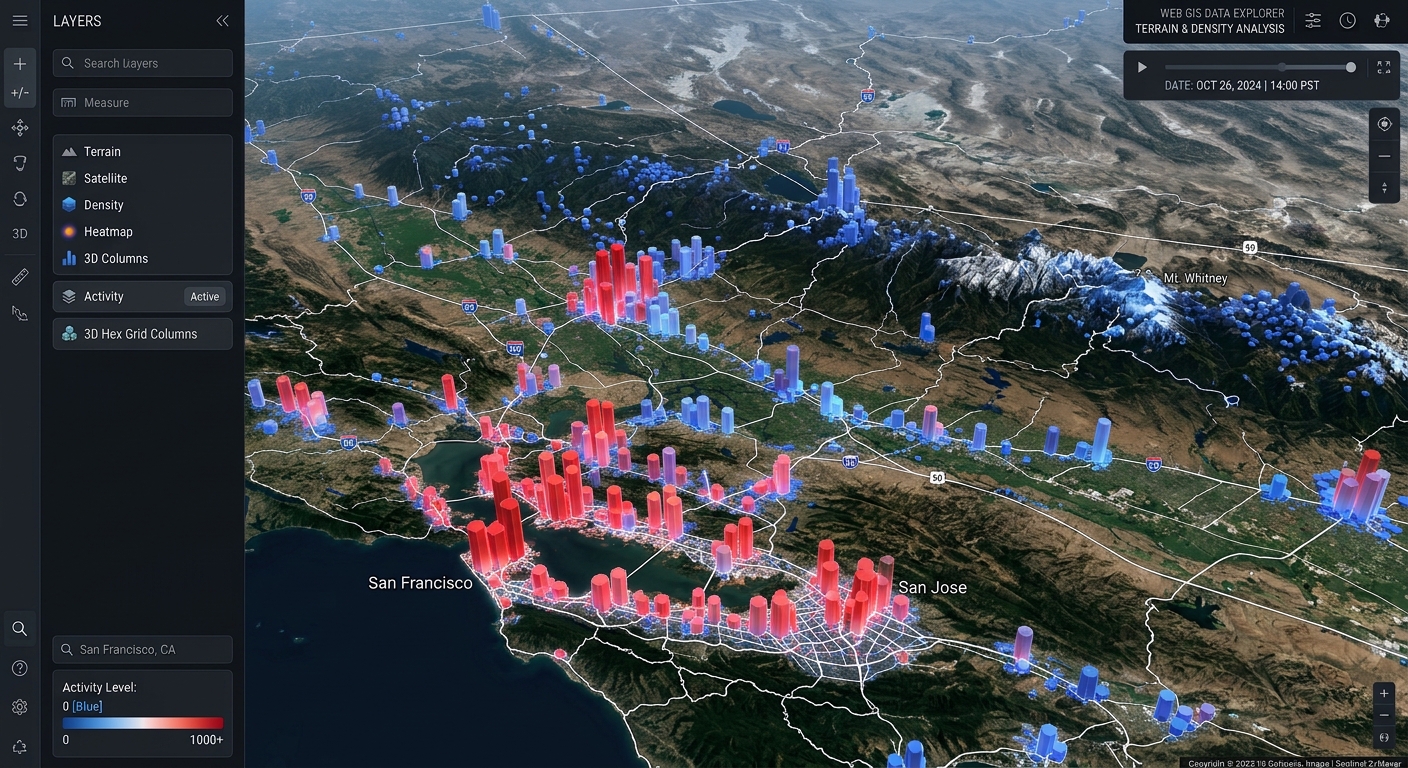
Creating 3D Web Scenes with Deck.gl and Mapbox GL JS
Introduction
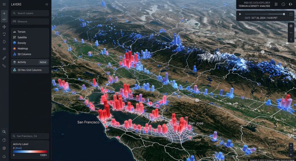
When you create 3D web scenes Deck.gl Mapbox GL JS, traditional two-dimensional maps often fall short when displaying massive spatial observations. Traditional web maps work well when displaying points, lines, and polygons in two dimensions. However, when a dataset contains hundreds of thousands of spatial observations, rendering every feature as an individual marker can overwhelm the visual display and consume substantial browser resources.
Imagine building a web GIS application to visualize road incidents, population density, flood reports, or infrastructure demand. A static point map may reveal where observations occur, but it often fails to communicate the intensity and spatial distribution of those observations clearly.
A better approach is to aggregate observations into three-dimensional hexagonal or rectangular cells, extrude geographic polygons, and combine these visualizations with a terrain basemap.
Two JavaScript libraries are particularly useful for this workflow:
-
Mapbox GL JS provides the interactive basemap, camera navigation, terrain, and map controls.
-
Deck.gl provides GPU-accelerated visualization layers, including
HexagonLayer,GridLayer, andGeoJsonLayer.
Deck.gl’s aggregation layers support GPU-based aggregation when the browser and selected layer configuration permit it. This can significantly improve performance compared with CPU-based aggregation, although actual performance still depends on the dataset, hardware, and rendering workload.
In this tutorial, we will build an interactive 3D web GIS scene with:
-
A Mapbox terrain basemap.
-
An angled camera with configurable pitch and bearing.
-
Asynchronous GeoJSON loading for point and polygon data.
-
Three-dimensional hexagon and grid aggregation.
-
Attribute-driven elevation and color.
-
Dynamic lighting and interactive hover feedback.
-
A synchronized Deck.gl overlay controlled by Mapbox navigation.
1. Set up the development environment
We will use a lightweight JavaScript project powered by Vite. This provides a development server and bundles the application for deployment.
1.1 Create the project
Install Node.js and npm, then run:
# Create a vanilla JavaScript project
npm create vite@latest deck-3d-scene -- --template vanilla

# Enter the project directory
cd deck-3d-scene

# Install the starter dependencies
npm install
Install Mapbox GL JS and the required Deck.gl modules:
npm install mapbox-gl \
  @deck.gl/core \
  @deck.gl/layers \
  @deck.gl/aggregation-layers \
  @deck.gl/mapbox
These packages provide the map renderer, core Deck.gl classes, GeoJSON rendering, aggregation layers, and Mapbox integration. The official Deck.gl documentation supports installing its individual modules through npm.
1.2 Organize the project
Use the following structure:
deck-3d-scene/
├── .env.local
├── index.html
├── public/
│   └── data/
│       ├── events.geojson
│       └── districts.geojson
└── src/
    ├── main.js
    └── style.css
The point dataset will be called events.geojson. The polygon dataset will be called districts.geojson.
For this example, we will assume the point features contain a numeric weight property, while polygons may contain height_m and risk_score properties. Adapt these field names to your own data.
1.3 Configure the Mapbox access token
Mapbox GL JS requires an access token to load Mapbox-hosted map styles and services. You can create a public token through the Mapbox account dashboard.
Create .env.local:
VITE_MAPBOX_ACCESS_TOKEN=pk.your_public_mapbox_token_hereReplace the placeholder with your actual public token.
Security note: A Vite variable prefixed with VITE_ is included in the client-side application. Use a public token with appropriate URL restrictions; never put a secret server-side token in browser code. Add .env.local to .gitignore so you do not commit your local configuration.
2. Create the HTML page
Replace the contents of index.html with the following code.
<!doctype html>
<html lang="en">
  <head>
    <meta charset="UTF-8" />

    <!-- Ensure the interface scales on mobile screens -->
    <meta name="viewport" content="width=device-width, initial-scale=1.0" />

    <title>3D Spatial Explorer</title>
  </head>

  <body>
    <header class="toolbar">
      <div>
        <h1>3D Spatial Explorer</h1>
        <p>Explore spatial intensity and polygon attributes</p>
      </div>

      <!-- Switch between hexagonal and rectangular aggregation -->
      <label for="aggregation-mode">
        Aggregation
        <select id="aggregation-mode">
          <option value="hexagon">3D Hexagons</option>
          <option value="grid">3D Grid</option>
        </select>
      </label>

      <!-- Updated by JavaScript during loading and error handling -->
      <span id="status" role="status" aria-live="polite">
        Initializing map…
      </span>
    </header>

    <!-- Mapbox renders the basemap; Deck.gl renders the data layers -->
    <main id="map" aria-label="Interactive three-dimensional spatial map">
      <div id="tooltip" class="tooltip" hidden></div>
    </main>

    <!-- Vite loads and bundles the application module -->
    <script type="module" src="/src/main.js"></script>
  </body>
</html>
The HTML defines the map container, aggregation selector, loading status, and a tooltip. The actual map and visualization layers will be initialized in JavaScript.
3. Style the map interface
Create src/style.css:
/* Use predictable sizing for the full application */
* {
  box-sizing: border-box;
}

html,
body {
  width: 100%;
  height: 100%;
  margin: 0;
  font-family: Inter, system-ui, -apple-system, sans-serif;
  color: #f1f5f9;
  background: #0b1220;
}

/* Header sits above the full-screen map */
.toolbar {
  position: relative;
  z-index: 10;
  display: flex;
  align-items: center;
  justify-content: space-between;
  gap: 1.25rem;
  min-height: 84px;
  padding: 12px 20px;
  background: #101a2b;
  border-bottom: 1px solid #25344a;
}

.toolbar h1 {
  margin: 0;
  font-size: 1.1rem;
}

.toolbar p {
  margin: 5px 0 0;
  color: #a9b8cb;
  font-size: 0.85rem;
}

.toolbar label {
  display: flex;
  align-items: center;
  gap: 10px;
  font-size: 0.9rem;
}

.toolbar select {
  padding: 9px 12px;
  border: 1px solid #42536b;
  border-radius: 6px;
  color: #f1f5f9;
  background: #1b2a40;
}

#status {
  max-width: 280px;
  color: #b7c7da;
  font-size: 0.8rem;
}

#status.error {
  color: #ffaaaa;
}

/* Map fills all available space below the toolbar */
#map {
  position: absolute;
  top: 84px;
  right: 0;
  bottom: 0;
  left: 0;
  overflow: hidden;
}

/* Tooltip uses map-local pixel coordinates */
.tooltip {
  position: absolute;
  z-index: 20;
  max-width: 240px;
  padding: 9px 12px;
  color: #ffffff;
  background: rgba(10, 18, 32, 0.95);
  border: 1px solid #526781;
  border-radius: 6px;
  font-size: 0.8rem;
  pointer-events: none;
  box-shadow: 0 4px 18px rgba(0, 0, 0, 0.25);
}

@media (max-width: 720px) {
  .toolbar {
    align-items: flex-start;
    flex-direction: column;
    gap: 10px;
  }

  #map {
    top: 155px;
  }

  #status {
    max-width: 100%;
  }
}
The #map element is the shared container for Mapbox GL JS. Its dimensions determine the size of the map viewport, while the tooltip is positioned relative to the same container.
The responsive styling is useful because 3D scenes can be particularly demanding on mobile devices, where memory and rendering performance may be more limited.
4. Initialize Mapbox GL JS with 3D terrain
Create src/main.js.
Begin by importing the libraries:
// Mapbox GL JS: interactive basemap and camera controls
import mapboxgl from "mapbox-gl";
import "mapbox-gl/dist/mapbox-gl.css";

// Deck.gl: synchronized rendering on the Mapbox map
import { MapboxOverlay } from "@deck.gl/mapbox";

// Standard vector and GeoJSON visualization
import { GeoJsonLayer } from "@deck.gl/layers";

// Aggregation layers for 3D density visualization
import {
  HexagonLayer,
  GridLayer
} from "@deck.gl/aggregation-layers";

// Lighting classes for shaded 3D geometry
import {
  AmbientLight,
  DirectionalLight,
  LightingEffect
} from "@deck.gl/core";

// Application styles
import "./style.css";
We import the modules individually so that the application has clear dependencies and does not rely on global library variables.
4.1 Read the configuration and initialize the map
Add the following code below the imports:
// Read configuration and interface elements.
const accessToken = import.meta.env.VITE_MAPBOX_ACCESS_TOKEN;
const statusElement = document.getElementById("status");
const tooltip = document.getElementById("tooltip");
const aggregationSelect = document.getElementById("aggregation-mode");

// Centralized helper for loading and error messages.
function setStatus(message, isError = false) {
  statusElement.textContent = message;
  statusElement.classList.toggle("error", isError);
}

// Stop early if the Mapbox token has not been configured.
if (!accessToken) {
  setStatus(
    "Missing Mapbox token. Configure VITE_MAPBOX_ACCESS_TOKEN.",
    true
  );

  throw new Error("Mapbox access token is missing.");
}

// Make the token available to Mapbox GL JS.
mapboxgl.accessToken = accessToken;

// Create the map with an oblique camera view.
const map = new mapboxgl.Map({
  container: "map",
  style: "mapbox://styles/mapbox/standard-satellite",
  center: [-122.4194, 37.7749],
  zoom: 11,
  pitch: 58,
  bearing: -24,
  maxPitch: 80,
  antialias: false
});

// Add native Mapbox camera controls.
map.addControl(new mapboxgl.NavigationControl(), "top-right");

// Add a scale indicator.
map.addControl(
  new mapboxgl.ScaleControl({
    maxWidth: 120,
    unit: "metric"
  }),
  "bottom-left"
);
Several settings are particularly important:
| Property | Purpose |
|---|---|
center |
Sets the initial longitude and latitude. |
zoom |
Determines the initial zoom level. |
pitch |
Tilts the camera to reveal 3D geometry. |
bearing |
Rotates the camera around the map. |
maxPitch |
Limits how far the camera can tilt. |
antialias |
Enables multisample anti-aliasing when supported; disabled here as a performance-conscious default. |
Mapbox GL JS supports setting the initial pitch and bearing when constructing a map. A nonzero pitch makes elevated columns and extruded geometry much easier to interpret.
The coordinates above are only an example. Replace them with the center of your study area.
4.2 Add the terrain elevation source
Mapbox terrain can be enabled by adding a raster digital elevation model (DEM) and passing its source ID to setTerrain().
Add this code:
// Add terrain after the map style has loaded.
map.on("style.load", () => {
  // Avoid adding the same source more than once.
  if (!map.getSource("mapbox-dem")) {
    map.addSource("mapbox-dem", {
      type: "raster-dem",
      url: "mapbox://mapbox.mapbox-terrain-dem-v1",
      tileSize: 512,
      maxzoom: 14
    });
  }

  // Apply the DEM as the map's elevation surface.
  map.setTerrain({
    source: "mapbox-dem",
    exaggeration: 1.25
  });
});

// Log rendering or network errors for debugging.
map.on("error", (event) => {
  if (event.error) {
    console.error("Mapbox GL JS error:", event.error);
  }
});
The exaggeration property increases the apparent relief of the terrain. A value of 1.25 is a starting point; adjust it to suit your geographic region and the scale of the map.
At this point, Mapbox handles the basemap, camera movements, terrain tiles, and map controls. The next step is to load your spatial data.
5. Load spatial point and polygon datasets asynchronously
For this tutorial, our data schema is:
Point features
{
  "type": "Feature",
  "geometry": {
    "type": "Point",
    "coordinates": [-122.4194, 37.7749]
  },
  "properties": {
    "weight": 4.2,
    "category": "high"
  }
}
Polygon features should contain numeric attributes such as:
{
  "properties": {
    "height_m": 80,
    "risk_score": 75
  }
}
The examples above illustrate the properties expected by the visualization. Your files must contain valid GeoJSON geometries and be saved as FeatureCollections in the public/data/ directory.
GeoJSON point coordinates use the order longitude, latitude, not latitude, longitude.
5.1 Create a reusable asynchronous loader
Add the following functions to main.js:
// Fetch a GeoJSON document and check the HTTP response.
async function fetchGeoJSON(url) {
  const response = await fetch(url);

  // Handle 404, 500, and other unsuccessful HTTP responses.
  if (!response.ok) {
    throw new Error(
      `Failed to fetch ${url}: HTTP ${response.status}`
    );
  }

  const geojson = await response.json();

  // Confirm that the file has the expected top-level structure.
  if (
    geojson.type !== "FeatureCollection" ||
    !Array.isArray(geojson.features)
  ) {
    throw new Error(`${url} is not a valid GeoJSON FeatureCollection.`);
  }

  return geojson;
}

// Convert point features into a flat array suitable for Deck.gl.
function normalizePointFeatures(geojson) {
  return geojson.features
    .filter((feature) => {
      return (
        feature?.geometry?.type === "Point" &&
        Array.isArray(feature.geometry.coordinates) &&
        feature.geometry.coordinates.length >= 2
      );
    })
    .map((feature, index) => {
      const [longitude, latitude] = feature.geometry.coordinates;

      // If weight is absent, treat each point as weight 1.
      const weight = Number(feature.properties?.weight ?? 1);

      // Discard invalid coordinates and invalid or negative weights.
      if (
        !Number.isFinite(longitude) ||
        !Number.isFinite(latitude) ||
        !Number.isFinite(weight) ||
        weight < 0
      ) {
        return null;
      }

      return {
        id: feature.id ?? index,
        position: [longitude, latitude],
        weight,
        properties: feature.properties ?? {}
      };
    })
    .filter(Boolean);
}
fetchGeoJSON() checks both the HTTP response and the data structure. normalizePointFeatures() converts GeoJSON point features into flat JavaScript objects containing a position and a numeric weight.
This preprocessing makes the later layer accessors simpler and guards against malformed records.
5.2 Store the loaded data
Add two variables:
// These are populated when asynchronous loading completes.
let pointData = [];
let polygonData = null;
We will load both files using Promise.all(). This allows the browser to request them concurrently rather than waiting for one download to finish before starting the other.
Note on large datasets: fetch() with response.json() is appropriate for many moderate datasets, including some datasets with hundreds of thousands of points. But downloading asynchronously does not make JSON parsing itself non-blocking. For very large datasets, streaming, spatial tiling, or worker-based processing may be necessary.
6. Configure dynamic lighting and polygon extrusions
Before configuring the aggregation layer, we will define a lighting effect and a polygon visualization.
6.1 Add a lighting effect
// Ambient light illuminates the geometry generally.
const ambientLight = new AmbientLight({
  color: [255, 255, 255],
  intensity: 0.7
});

// Directional light adds stronger shading from one direction.
const directionalLight = new DirectionalLight({
  color: [255, 255, 255],
  intensity: 0.9,
  direction: [-1, -3, -1]
});

// Bundle the light sources into a Deck.gl effect.
const lightingEffect = new LightingEffect({
  ambientLight,
  directionalLights: [directionalLight]
});
Ambient light reduces overly dark surfaces, while directional lighting makes the vertical sides and tops of extruded cells easier to distinguish.
6.2 Create attribute-driven polygon styles
We will assign polygon color based on risk_score and height based on height_m. If height_m is missing or invalid, we will derive a simple illustrative height from risk_score.
// Convert a risk score from 0-100 into an RGB color.
function getRiskColor(feature) {
  const raw = Number(feature.properties?.risk_score);
  const risk = Number.isFinite(raw)
    ? Math.max(0, Math.min(100, raw))
    : 35;

  // Normalize the score into the interval 0-1.
  const t = risk / 100;

  // Low scores are blue; high scores are red.
  return [
    Math.round(40 + 205 * t),
    Math.round(150 - 95 * t),
    Math.round(230 - 185 * t),
    180
  ];
}

// Get a polygon's height for 3D extrusion.
function getPolygonElevation(feature) {
  const measuredHeight = Number(feature.properties?.height_m);

  // Use a valid supplied height when possible.
  if (Number.isFinite(measuredHeight)) {
    return Math.max(0, measuredHeight);
  }

  // Otherwise use risk score as an illustrative extrusion height.
  const risk = Number(feature.properties?.risk_score);

  if (Number.isFinite(risk)) {
    return Math.max(0, Math.min(100, risk)) * 8;
  }

  return 0;
}
The color function normalizes the score and interpolates between blue and red. The elevation function prefers a supplied height, making the visualization easier to interpret when actual height measurements exist.
The fallback height is a visual encoding—not a claim that the polygon is physically that tall.
6.3 Build the polygon layer
We will use GeoJsonLayer, which supports polygon extrusion through extruded and getElevation.
function createPolygonLayer() {
  return new GeoJsonLayer({
    id: "districts-3d",
    data: polygonData,

    // Draw filled polygon surfaces and their outlines.
    filled: true,
    stroked: true,
    getLineColor: [225, 235, 245, 200],
    getLineWidth: 1,
    lineWidthUnits: "pixels",

    // Turn polygons into three-dimensional extrusions.
    extruded: true,
    getElevation: getPolygonElevation,

    // Encode risk in polygon color.
    getFillColor: getRiskColor,

    // Apply shading to the extruded geometry.
    material: true,

    // Partial transparency retains visual context from the basemap.
    opacity: 0.75,

    // The polygon layer is contextual, so it does not capture the tooltip.
    pickable: false
  });
}
A polygon with a higher risk_score will be redder. A polygon with a higher height_m will extend farther above its coordinate plane.
For a real-world application, choose an elevation scale appropriate to the data units. For example, a real building height in meters should not be treated as a population count or a risk score without a deliberate visual transformation.
7. Build a Deck.gl HexagonLayer for 3D density
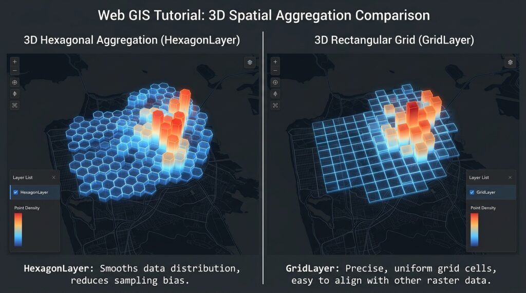
The HexagonLayer aggregates points into hexagonal cells. Each cell can receive a color and height based on the attributes of the observations falling within it.
The layer supports built-in aggregation methods such as SUM, MEAN, MIN, MAX, and COUNT. It can perform aggregation on the GPU when the configuration permits it.
7.1 Define a shared color scale
// RGB colors, ordered from low to high aggregate weight.
const densityColorRange = [
  [35, 80, 210],
  [40, 160, 220],
  [70, 200, 120],
  [250, 190, 60],
  [220, 55, 55]
];
We will use blue and green for lower values and yellow and red for higher aggregate values.
7.2 Configure the HexagonLayer
Add this function to main.js:
function createHexagonLayer() {
  return new HexagonLayer({
    id: "event-hexagons",
    data: pointData,

    // Aggregate on the GPU when supported by this configuration.
    gpuAggregation: true,

    // Read geographic coordinates from each point.
    getPosition: (d) => d.position,

    // Use the weight attribute to determine cell color.
    getColorWeight: (d) => d.weight,
    colorAggregation: "SUM",
    colorRange: densityColorRange,

    // Use the number of points to determine cell height.
    getElevationWeight: 1,
    elevationAggregation: "COUNT",

    // Extrude cells into three dimensions.
    extruded: true,

    // Hexagon radius is specified in meters.
    radius: 400,
    coverage: 0.88,

    // Map elevation counts into a visible height range.
    elevationRange: [0, 1200],
    elevationScale: 1,

    // Enable material shading and hover interactions.
    material: {
      ambient: 0.35,
      diffuse: 0.6,
      shininess: 32,
      specularColor: [0.3, 0.3, 0.3]
    },

    pickable: true,
    autoHighlight: true,
    opacity: 0.88,

    // Handle hover feedback.
    onHover: handleLayerHover
  });
}
Here is how the main properties work:
| Property | Meaning |
|---|---|
getPosition |
Returns the coordinates of each observation. |
getColorWeight |
Supplies the numeric attribute used for color aggregation. |
colorAggregation: "SUM" |
Sums weight values inside each cell. |
getElevationWeight: 1 |
Gives each observation an equal elevation weight. |
elevationAggregation: "COUNT" |
Makes cell height represent the number of points. |
radius |
Sets the hexagon radius in meters. |
elevationRange |
Maps aggregated counts to the visual elevation range. |
coverage |
Controls the visible size of the hexagons relative to their bin radius. |
pickable |
Allows user interaction with the generated cells. |
This configuration intentionally separates color from height. A cell can be tall because it contains many observations, while its color represents the sum of their weights. That is useful when visualizing both event frequency and event magnitude.
The radius affects how points are grouped spatially. A smaller radius provides finer spatial detail, while a larger radius creates broader patterns with fewer cells.
8. Create an alternative GridLayer
A rectangular grid offers an alternative view of the same points. GridLayer exposes a similar aggregation interface, but uses square cells with a configurable cell size in me
Add this function:
function createGridLayer() {
  return new GridLayer({
    id: "event-grid",
    data: pointData,

    gpuAggregation: true,

    // Return the point coordinates.
    getPosition: (d) => d.position,

    // Color encodes the sum of each cell's weights.
    getColorWeight: (d) => d.weight,
    colorAggregation: "SUM",
    colorRange: densityColorRange,

    // Height encodes the number of points.
    getElevationWeight: 1,
    elevationAggregation: "COUNT",

    // Set rectangular cell dimensions.
    cellSize: 500,

    // Configure 3D extrusion and its visual range.
    extruded: true,
    elevationRange: [0, 1200],
    elevationScale: 1,

    material: {
      ambient: 0.35,
      diffuse: 0.6,
      shininess: 32,
      specularColor: [0.3, 0.3, 0.3]
    },

    pickable: true,
    autoHighlight: true,
    opacity: 0.88,

    onHover: handleLayerHover
  });
}
Choose between the layers according to the analytical goal:
-
HexagonLayeris useful for density patterns and spatial clustering. -
GridLayeris useful when rectangular bins correspond more naturally to an analytical grid or reporting framework.
Both aggregate points into cells, reducing the need to draw every observation separately as an individually visible marker.
9. Add interactive hover feedback
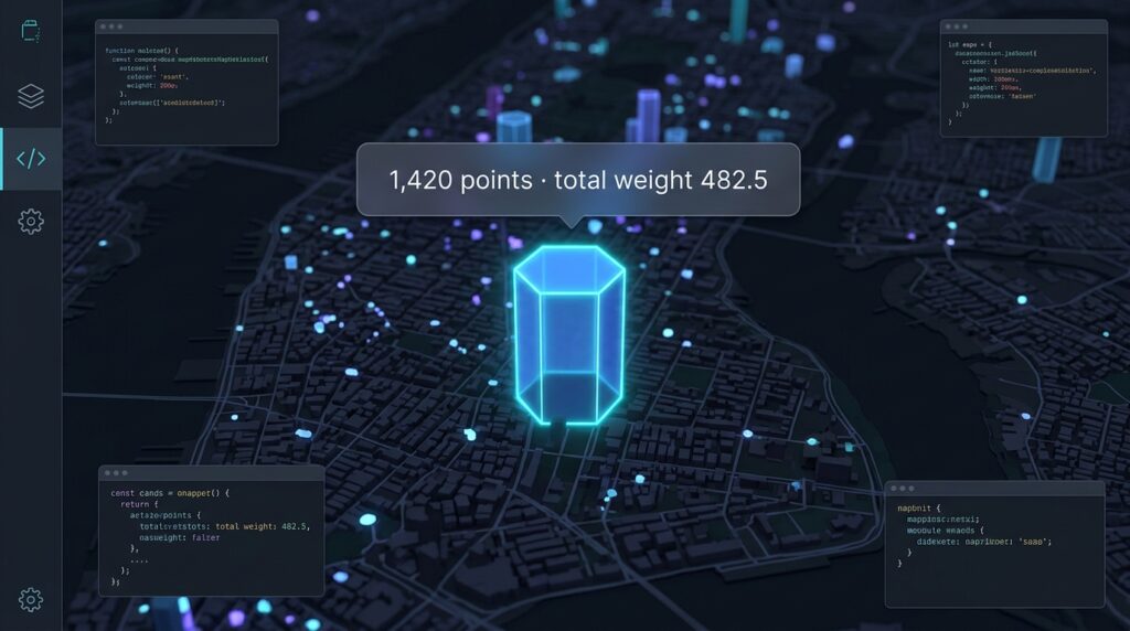
A useful 3D web scene should let users inspect the values behind the visualization.
Add this function:
function handleLayerHover({ object, x, y }) {
  // Hide the tooltip when the pointer leaves an interactive cell.
  if (!object) {
    tooltip.hidden = true;
    return;
  }

  // Read aggregated properties returned by the layer.
  const count = Number(object.count ?? 0);
  const totalWeight = Number(object.colorValue ?? 0);

  tooltip.textContent =
    `${count.toLocaleString()} points · ` +
    `total weight ${totalWeight.toFixed(1)}`;

  // Keep the tooltip inside the map viewport.
  const mapWidth = map.getContainer().clientWidth;
  const mapHeight = map.getContainer().clientHeight;

  const left = Math.max(
    8,
    Math.min(x + 12, mapWidth - 250)
  );

  const top = Math.max(
    8,
    Math.min(y + 12, mapHeight - 50)
  );

  tooltip.style.left = `${left}px`;
  tooltip.style.top = `${top}px`;
  tooltip.hidden = false;
}
When the user hovers over an aggregated cell, the tooltip displays the number of observations and the summed weight. Both values help explain the visual encodings.
The exact picking information available depends on the layer and aggregation configuration; the HexagonLayer documentation describes the aggregated object and its count and color/elevation values.
10. Connect Deck.gl to the Mapbox camera
The important integration component is MapboxOverlay.
Rather than constructing an independent Deck.gl map with a separate camera, we attach the overlay to the existing Mapbox map. This allows Deck.gl to synchronize its rendering with Mapbox’s camera navigation. The integration supports both overlaid and interleaved modes.
10.1 Build the layer collection
Add this function:
function buildLayers(mode) {
  const layers = [];

  // Add polygons first so they provide contextual geography.
  if (polygonData) {
    layers.push(createPolygonLayer());
  }

  // Add exactly one aggregation layer.
  if (pointData.length > 0) {
    if (mode === "grid") {
      layers.push(createGridLayer());
    } else {
      layers.push(createHexagonLayer());
    }
  }

  return layers;
}
This function returns a layer array that can be submitted to Deck.gl. The selected aggregation mode determines which density layer is rendered.
10.2 Create the MapboxOverlay and load the data
Add the final initialization block:
// Wait until Mapbox has finished its initial load.
map.once("load", async () => {
  // Use interleaved rendering to share Mapbox's WebGL2 context.
  const deckOverlay = new MapboxOverlay({
    interleaved: true,
    layers: [],
    effects: [lightingEffect]
  });

  // Register the overlay as a Mapbox control.
  map.addControl(deckOverlay);

  try {
    setStatus("Loading spatial datasets…");

    // Fetch both datasets concurrently.
    const [eventsGeoJSON, districtsGeoJSON] = await Promise.all([
      fetchGeoJSON("/data/events.geojson"),
      fetchGeoJSON("/data/districts.geojson")
    ]);

    // Normalize point records for the aggregation layers.
    pointData = normalizePointFeatures(eventsGeoJSON);

    // Preserve the polygon FeatureCollection for GeoJsonLayer.
    polygonData = districtsGeoJSON;

    if (pointData.length === 0) {
      throw new Error("No valid point features were found.");
    }

    // Render the initial layer configuration.
    deckOverlay.setProps({
      layers: buildLayers(aggregationSelect.value)
    });

    setStatus(
      `Loaded ${pointData.length.toLocaleString()} points and ` +
      `${polygonData.features.length.toLocaleString()} polygons.`
    );
  } catch (error) {
    console.error("Spatial data loading failed:", error);

    setStatus(
      `Could not load spatial data: ${error.message}`,
      true
    );
  }

  // Update the visualization when the dropdown changes.
  aggregationSelect.addEventListener("change", () => {
    deckOverlay.setProps({
      layers: buildLayers(aggregationSelect.value)
    });
  });
});
This is where the application comes together.
-
The map finishes initializing.
-
A Deck.gl overlay is attached to Mapbox.
-
The two datasets are fetched concurrently.
-
Point records are normalized.
-
The polygon and selected aggregation layers are created.
-
The overlay renders the layers in synchronization with the map.
-
Changing the dropdown swaps the current aggregation layer without creating a second map.
The official integration documentation identifies MapboxOverlay as the recommended integration for applications that want Deck.gl layers within the Mapbox ecosystem. In interleaved mode, Deck.gl layers share Mapbox’s WebGL2 context and can participate in layer ordering and 3D occlusion.
10.3 Run the application
Start the Vite development server:
npm run devOpen the local address printed by Vite in your browser.
For the application to display data, ensure that both files exist at:
public/data/events.geojson
public/data/districts.geojson
If the map loads but your data does not appear, inspect the browser console for fetch errors, geometry issues, or unexpected attribute values.
11. Understanding the 3D scene’s rendering modes
You will see this configuration in the overlay:
const deckOverlay = new MapboxOverlay({
  interleaved: true,
  layers: [],
  effects: [lightingEffect]
});
The interleaved option changes how Deck.gl is rendered alongside the basemap.
| Mode | Rendering behavior | Appropriate use |
|---|---|---|
interleaved: true |
Renders Deck.gl layers in Mapbox’s WebGL2 context and layer stack. | When the visual scene requires integrated layer ordering or 3D occlusion. |
interleaved: false |
Uses a separate Deck.gl canvas above the Mapbox map. | When interleaving is unnecessary or when overlay compatibility is more important. |
With interleaving enabled, Deck.gl layers can be placed in relation to Mapbox style layers where supported, so certain objects can appear behind labels or interact correctly with 3D scene depth. The mode requires a compatible WebGL2 environment.
Important terrain limitation: Deck.gl’s Mapbox integration has partial terrain support. The cameras can be synchronized, but Deck.gl geometry positioned at z = 0 is rendered at sea level rather than automatically following the Mapbox terrain surface.
Consequently, the 3D hexagons in this tutorial are data extrusions, not terrain-draped hexagons. In steep terrain, they may appear below or out of alignment with the ground surface. For a terrain-conforming analysis, you must account for the underlying elevation—for example, by sampling elevation data and preparing appropriate 3D
12. Performance optimization for high-performance web GIS 3D
GPU acceleration helps, but it does not eliminate all browser constraints. The most effective strategy is to reduce unnecessary work before and during rendering.
12.1 Keep aggregation on the GPU where possible
In this tutorial, the aggregation layers use:
gpuAggregation: true,
getColorWeight: (d) => d.weight,
colorAggregation: "SUM",
getElevationWeight: 1,
elevationAggregation: "COUNT"
These built-in accessors use supported aggregation operations, allowing GPU aggregation in compatible configurations.
Be aware that custom getColorValue or getElevationValue callbacks disable GPU aggregation for these layers. That can be reasonable for specialized statistics, but it should be a deliberate trade-off.
12.2 Avoid rebuilding layers on every camera movement
A common mistake is to reconstruct the entire dataset or the Deck.gl layer array every time the Mapbox camera changes.
For example, avoid attaching code like this to a move event:
// Avoid this pattern for large, unchanged datasets.
map.on("move", () => {
  deckOverlay.setProps({
    layers: buildLayers(aggregationSelect.value)
  });
});
The Mapbox overlay already synchronizes rendering with camera movement. Recreating layers unnecessarily can trigger additional processing and resource uploads.
Instead, update the layers when the data changes, when the user switches modes, or when a relevant visualization setting changes. Deck.gl’s performance guidance emphasizes minimizing data changes and layer updates because buffer generation and uploading may be expensive for large inputs.
12.3 Keep the rendered geometry manageable
A few practical adjustments make a difference:
-
Increase
radiusorcellSizewhen a more generalized density surface is sufficient. -
Use the polygon level of detail appropriate to the current zoom level.
-
Simplify large polygon geometries before transmitting them to the browser.
-
Avoid rendering every point as a separate 3D mesh when aggregation communicates the required information.
-
Reduce unnecessary transparency, effects, and excessive vertical exaggeration if rendering becomes slow.
Remember that a large point dataset and a large polygon dataset have different costs. GPU aggregation may reduce the visual complexity of the points, but it does not automatically simplify the polygon geometries in GeoJsonLayer.
12.4 Stream and partition data carefully
Loading a single GeoJSON FeatureCollection is convenient for a demonstration, but large files can consume substantial memory during download, parsing, normalization, and GPU buffer generation.
For much larger or continuously changing datasets, consider:
Spatial filtering on the server. Return only records intersecting the current study area or viewport rather than downloading the entire dataset.
Vector tiles. Serve pre-tiled features and request only the tiles visible at the current zoom. Deck.gl includes a MVTLayer for rendering Mapbox Vector Tiles; this is available through its Geo-layer package.
Binary formats and workers. Formats such as Apache Arrow or custom binary layouts can reduce JSON processing overhead. Deck.gl’s performance documentation also describes transferring typed arrays and preparing data in workers for demanding applications.
Batched updates. If data arrives continuously, accumulate changes and update the visualization at controlled intervals. Appending one record and rebuilding the aggregate layer for every incoming event can be more expensive than batching the updates.
The best choice depends on whether the application is primarily a static density map, a live monitoring dashboard, or a high-volume analytical system.
12.5 Monitor browser and GPU limitations
Mapbox GL JS requires WebGL2 support, and the browser must have hardware acceleration available for the best experience.
Test the application on realistic devices, especially if users will access it on mobile. Start with a representative portion of your dataset and gradually increase its size while monitoring loading time, responsiveness, memory pressure, and rendering quality.
13. Troubleshooting
| Problem | Likely cause | What to check |
|---|---|---|
| Map tiles fail to load | Missing or restricted access token | Check .env.local and token URL restrictions. |
| Map appears but data is absent | Incorrect file path or invalid GeoJSON | Open the two data URLs directly and inspect the console. |
| No visible 3D columns | extruded is false or elevation values are zero |
Check extruded, elevationRange, and the aggregated values. |
| Cells appear too tall | Height range is excessive for the density distribution | Reduce elevationRange or adjust the weight semantics. |
| Scene is sluggish | Excessive geometry, frequent data updates, or GPU/memory constraints | Simplify polygons, increase cell size, filter data, and minimize updates. |
| Deck.gl geometry is misaligned with terrain | The overlay’s geometry is not automatically draped over Mapbox terrain | Sample terrain elevation or use a terrain-aware rendering workflow. |
Conclusion
Creating 3D Web Scenes with Deck.gl and Mapbox GL JS involves more than displaying an angled basemap. The strength of the combination is that Mapbox handles navigation and geographic context while Deck.gl provides specialized layers for turning large spatial datasets into interactive visual summaries.
The core workflow is:
GeoJSON datasets
      ↓
Async loading and validation
      ↓
Mapbox GL JS
      ├── Basemap
      ├── Camera navigation
      └── 3D terrain
              ↓
       MapboxOverlay
              ↓
          Deck.gl
          ├── GeoJsonLayer
          ├── HexagonLayer
          ├── GridLayer
          └── Lighting and interactions
              ↓
      Interactive 3D web GIS
For large point datasets, HexagonLayer and GridLayer are useful because they aggregate observations into cells whose color and height can represent different attributes. GeoJsonLayer provides a complementary way to extrude polygon data.
For demanding applications, the most important performance decisions often concern data delivery, geometry complexity, GPU aggregation, and how frequently the application updates its layers.
Finally, remember that synchronized cameras and a 3D terrain basemap do not automatically make every Deck.gl feature conform to the terrain surface. A production application that relies on ground-level placement must address that distinction explicitly.