
Geographically Weighted Principal Component Analysis (GWPCA) in GIS
Introduction: Why Spatial Data Needs Local Multivariate Analysis

Principal Component Analysis (PCA) is a multivariate statistical technique used to reduce a large set of correlated variables into a smaller number of components that summarize the dominant patterns of variation in the data. It is widely used in environmental science, urban studies, remote sensing, public health, and socioeconomic research.
However, geographic datasets introduce an important complication: relationships among variables may differ from one location to another.
Consider a study of urban socioeconomic conditions using census data. Household income, unemployment, educational attainment, housing costs, and population age structure may describe one dominant dimension of urban inequality in a central business district, but a different dimension in a suburban or industrial region.
A conventional global PCA calculates one covariance or correlation structure for the entire dataset. It provides a single set of principal components that summarizes the overall pattern. If the multivariate structure genuinely varies across space, that global summary can obscure important local differences.
Geographically Weighted Principal Component Analysis (GWPCA) addresses this issue by calculating a locally weighted PCA around each observation location. Nearby observations receive greater weight than distant observations, allowing the principal component loadings, eigenvalues, and explained variance to vary spatially. GWPCA is therefore useful for exploring spatial non-stationarity in multivariate relationships. By capturing spatial heterogeneity, Geographically Weighted Principal Component Analysis provides significantly deeper insights than traditional global reduction techniques.
Global PCA
All observations contribute to one global covariance or correlation matrix.
One component structure
Global loadings and eigenvalues
GWPCA
Each evaluation location uses a distance-weighted neighborhood.
Local component structures
Spatially varying loadings and eigenvalues
Conceptual comparison. Local PCA structures are estimated from overlapping neighborhoods, not from independent, non-overlapping geographic zones.
It is important to make one methodological distinction. Global PCA does not explicitly test or impose a spatial stationarity assumption in the same way as a spatial regression model. Rather, applying ordinary PCA to a spatial dataset produces a single global component structure. GWPCA is useful when that global structure may be an inadequate summary of geographic variation.
This tutorial develops the theory, explains spatial weighting and bandwidth selection, and demonstrates how to run and interpret GWPCA using R and the GWmodel package.
1. Core Concepts of Geographically Weighted PCA
1.1 Global PCA as the starting point
Suppose a geographic dataset contains \(n\) observations and \(p\) numeric variables. These could be census areas characterized by unemployment, income, education, housing costs, and age composition.
The data matrix is:
Conventional PCA typically centers the variables and, when units differ, standardizes them before calculating the covariance or correlation matrix.
The resulting eigenvalue decomposition is:
where:
-
\(\mathbf{S}\) is the global covariance or correlation matrix.
-
\(\lambda_k\) is the eigenvalue for component \(k\).
-
\(\mathbf{v}_k\) is the corresponding eigenvector, which defines the component direction.
The first principal component (PC1) explains the largest possible proportion of total variance among all linear combinations of the variables. The second explains the largest remaining proportion subject to being orthogonal to the first, and so forth.
The difficulty is that one global matrix describes the multivariate structure across all observations. When relationships vary geographically, that matrix may conceal contrasts between local populations or environments.
1.2 What makes PCA geographically weighted?
GWPCA replaces the single global covariance structure with a sequence of local weighted covariance structures.
At each evaluation location \(s_i\), the method gives greater importance to observations near that location and less importance to more distant observations. A separate PCA is then calculated using the resulting local weights.
The process produces:
-
Local eigenvalues, indicating the amount of local variance captured by each component.
-
Local eigenvectors or loadings, describing how the input variables contribute to the components locally.
-
Local explained-variance percentages, showing how much of the local multivariate variation is summarized by each component.
-
Local scores, when requested, expressing observations in their corresponding local component coordinate systems.
The GWmodel package implements basic and robust GWPCA, offers bandwidth selection through cross-validation, and returns location-specific loadings and explained-variance information.
1.3 Moving spatial weighting matrices and kernel functions
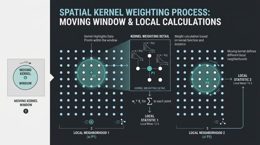
The defining mechanism of GWPCA is the spatial weighting scheme. For an evaluation location \(s_i\), the weight assigned to observation \(j\) can be written as:
where:
-
\(d_{ij}\) is the geographic distance between observations \(i\) and \(j\).
-
\(h_i\) is the bandwidth, which determines the spatial extent of the neighborhood.
-
\(K(\cdot)\) is the kernel function used to convert distance into a weight.
An observation near the evaluation location may receive a weight close to 1, while more distant observations receive smaller weights or zero weights, depending on the kernel.
At a high level, the local weighting matrix describes how much influence each observation has when estimating the local PCA at a particular location.
Common kernel functions
| Kernel | Weighting behavior | Main consideration |
|---|---|---|
| Gaussian | Decreases smoothly with distance; theoretical support extends indefinitely | Distant observations retain small positive weights |
| Exponential | Decreases exponentially with distance | Smooth distance decay |
| Bisquare | Declines to zero at the bandwidth boundary | Excludes observations outside the effective bandwidth |
| Tricube | Smoothly declines to zero at the bandwidth boundary | Gives a localized neighborhood with gradual tapering |
| Boxcar | Equal weights inside the bandwidth and zero outside | Abrupt neighborhood boundary |
For example, the bisquare kernel used by GWmodel follows:
A kernel does not determine the analytical scale on its own; bandwidth selection is equally important. A broad bandwidth produces a more geographically smoothed component structure, while a narrow bandwidth permits more localized variation.
1.4 Local means and covariance matrices
At each evaluation location \(s_i\), GWPCA calculates weighted local statistics. For variable \(a\), the weighted local mean can be expressed as:
Using the local means, the local weighted covariance matrix can be written conceptually as:
Here, \(\mathbf{x}_j\) is the vector of attributes at observation \(j\), and \(\bar{\mathbf{x}}_i\) is the vector of locally weighted means.
This equation illustrates the principle. Particular implementations may use different variance normalizations or robust estimators, so the exact numerical results depend on the software and settings.
PCA is then performed on the local matrix:
Both the eigenvalue \(\lambda_{ik}\) and the component direction \(\mathbf{v}_{ik}\) can now vary with location.
This is the essence of local PCA for spatial statistics: the analysis investigates how the multivariate relationships differ across geographic neighborhoods rather than treating the entire study area as one statistically homogeneous system.
1.5 Interpreting local eigenvalues and eigenvectors
Eigenvalues and eigenvectors answer different questions.
Local eigenvalues quantify the variance represented by individual local components. A large first eigenvalue relative to the sum of the local eigenvalues indicates that PC1 captures a substantial share of the locally observed multivariate variation.
Local eigenvectors or loadings describe the direction of each component in the input-variable space. They help reveal which variables contribute most strongly to a component and whether the local combination differs across regions.
Suppose the variables are income, unemployment, educational attainment, and housing costs. The first component may be associated primarily with employment and education in one area, but have stronger contributions from housing costs and income in another.
Such a pattern can suggest different dimensions of socioeconomic structure. Its actual interpretation must, however, be determined from the local loading patterns, variable definitions, and geographic context rather than assumed in advance.
2. Step-by-Step Practical Workflow in R
This workflow uses polygon-based census data, although GWPCA can also be applied to spatial point observations. The example investigates whether demographic indicators have different multivariate structures across an urban study area.
We will use:
-
sffor reading and managing spatial features. -
GWmodelfor GWPCA and bandwidth selection. -
ggplot2for mapping local results.
The GWmodel documentation confirms that its GWPCA functions support spatial data objects, including sf, and can return local variance proportions and loading information.
Step 1 — Prepare the spatial attribute table
Start with a polygon layer where each feature represents a census tract or another geographic reporting unit. Each row should contain the geometry and its associated demographic attributes.
For this example, suppose the input data contains:
| Variable | Description | Suggested interpretation |
|---|---|---|
pct_under15 |
Percentage of residents below age 15 | Younger population structure |
pct_over65 |
Percentage of residents aged 65 or above | Older population structure |
median_income |
Median household income | Economic conditions |
unemployment_rate |
Unemployment rate | Labor-market conditions |
rent_burden |
Share of households with high housing costs | Housing affordability |
bachelor_plus |
Percentage with a bachelor’s degree or higher | Educational attainment |
These are illustrative field names. Replace them with the actual column names in your census dataset.
Data preparation requirements
-
Ensure that each geographic unit has one consistent set of demographic attributes.
-
Prefer rates, proportions, and suitable normalized indicators over raw population counts when population size is not itself the variable of interest.
-
Check missing values, invalid values, duplicate records, extreme outliers, and variables with zero or near-zero variance.
-
Review correlations and avoid including redundant variables without a substantive reason.
-
Transform strongly skewed variables where appropriate, such as household income, before calculating PCA.
-
Use comparable variable definitions and reference periods across all areas.
For polygon data, the location of each observation must also be defined. GWmodel can use polygon centroids as evaluation locations when working with sf polygons. If the polygons are highly irregular or their centroids fall outside their boundaries, consider whether an alternative representative location is more appropriate for the research design.
Step 2 — Install and load the R packages
Install the required packages once:
install.packages(c(
  "sf",
  "GWmodel",
  "ggplot2"
))
Load them in your analysis script:
library(sf)
library(GWmodel)
library(ggplot2)
The GWmodel package includes functions for geographically weighted methods, including gwpca() for local principal component analysis and bw.gwpca() for bandwidth selection. Its current documentation describes bandwidth selection using cross-validation.
Step 3 — Read and validate the spatial dataset
Read the input layer from a GeoPackage:
dat <- st_read(
  "urban_demographics.gpkg",
  layer = "tracts",
  quiet = TRUE
)

# Choose the demographic variables for analysis.
vars <- c(
  "pct_under15",
  "pct_over65",
  "median_income",
  "unemployment_rate",
  "rent_burden",
  "bachelor_plus"
)

# Check that all requested attributes exist.
missing_vars <- setdiff(vars, names(dat))

if (length(missing_vars) > 0) {
  stop(
    "Missing variables: ",
    paste(missing_vars, collapse = ", ")
  )
}

# Verify that the spatial data has a CRS.
if (is.na(st_crs(dat))) {
  stop("The dataset has no defined coordinate reference system.")
}

# Check that all analysis variables are numeric.
attributes <- st_drop_geometry(dat)[, vars, drop = FALSE]

if (!all(vapply(attributes, is.numeric, logical(1)))) {
  stop("All GWPCA input variables must be numeric.")
}
Now check the coordinate system.
st_crs(dat)
st_is_longlat(dat)
Use an appropriate projected coordinate reference system for a local urban study whenever possible. This allows the spatial weighting process to use meaningful planar distances, typically in meters. Select the projection according to the study area’s location and extent rather than choosing an arbitrary CRS.
For example, if the source layer uses longitude and latitude, transform it to a locally appropriate projected CRS before calculating planar distances:
# Example only: replace with the correct projected EPSG
# code for your study area.
#
# dat <- st_transform(dat, YOUR_PROJECTED_EPSG)
The placeholder must be replaced with a valid CRS identifier before the code is executed. Alternatively, GWPCA supports great-circle distance calculations through longlat = TRUE, which can be appropriate for longitude–latitude data. In either case, the distance configuration must match the coordinate system.
Step 4 — Handle missing values and low-variance variables
GWPCA requires suitable numeric values for the selected variables. Missing values can undermine local covariance calculations, particularly when different variables have missing records across the study area.
For a simple, transparent baseline, retain observations with complete data for all analysis variables:
attributes <- st_drop_geometry(dat)[, vars, drop = FALSE]

complete <- complete.cases(attributes)

dat <- dat[complete, ]

attributes <- st_drop_geometry(dat)[, vars, drop = FALSE]

# Inspect variable standard deviations.
variable_sd <- vapply(
  attributes,
  sd,
  numeric(1)
)

print(variable_sd)

if (any(!is.finite(variable_sd) | variable_sd == 0)) {
  stop(
    "Remove or investigate variables with zero ",
    "or non-finite variance."
  )
}
Complete-case analysis is easy to implement, but it can introduce bias when missing data are systematically associated with geography or socioeconomic conditions. For serious research, investigate missingness patterns and justify any imputation or record-exclusion procedure.
Also inspect the variable distributions and correlation matrix:
summary(attributes)

cor(
  attributes,
  use = "pairwise.complete.obs"
)
The correlation matrix is a diagnostic tool for understanding redundancy and potential collinearity. It does not establish that every highly correlated pair must be removed; the decision should be guided by the substantive meaning of the indicators.
Why standardization matters
Income may be measured in currency units, while unemployment and demographic proportions are recorded as percentages. Variables with larger numerical scales can dominate an unstandardized PCA.
In GWmodel, the scaling = TRUE argument standardizes the variables before the local analysis. This is a sensible default for the mixed demographic indicators in this example. The global PCA used for comparison should apply consistent centering and scaling so that the results are comparable.
Step 5 — Establish a global PCA baseline
Before running GWPCA, calculate an ordinary PCA. This provides a useful point of comparison for determining whether the locally varying component structures reveal information that a global analysis conceals.
global_pca <- prcomp(
  attributes,
  center = TRUE,
  scale. = TRUE
)

summary(global_pca)

# Global loadings for the first principal component.
global_loadings_pc1 <- global_pca$rotation[, 1]

print(global_loadings_pc1)
The output contains one global set of component loadings and variance proportions.
Inspect the first component and determine which indicators contribute most strongly to it. For example, if economic indicators dominate PC1 across the entire dataset, the global result may suggest that economic conditions provide the principal dimension of multivariate variation.
However, this interpretation may be incomplete if demographic structures differ between the city center, industrial areas, and suburban neighborhoods. GWPCA helps investigate that possibility.
Step 6 — Select an appropriate spatial bandwidth
Bandwidth selection is one of the most influential decisions in GWPCA. It determines the geographic scale at which local PCA is calculated.
Two main options are available.
Fixed-distance bandwidth
A fixed bandwidth uses one distance threshold throughout the study area. Each local analysis draws on observations within the specified distance, with their weights determined by the kernel.
This approach is attractive when the sampling locations are reasonably evenly spaced and the same geographic radius has substantive meaning across the study area.
Its disadvantage is that neighborhoods with sparse observations may contain too little local information, while dense areas may include many observations.
Adaptive bandwidth
An adaptive bandwidth is based on a specified number of nearby observations. The geographic radius expands in sparse regions and contracts in dense regions, maintaining a more consistent local sample size.
This is often useful for census datasets with irregular spatial density. In GWmodel, the adaptive = TRUE option indicates an adaptive neighborhood size rather than a
Choosing the bandwidth strategy
Fixed
One distance threshold
Useful when observations are regularly distributed and a consistent geographic radius makes sense.
Adaptive
A selected neighborhood size
Useful when the sampling density varies substantially between urban centers and peripheral areas.
Automatically select a bandwidth with bw.gwpca()
GWmodel provides a bandwidth-selection function that uses cross-validation. The following example searches for an adaptive bisquare bandwidth for a two-component GWPCA:
set.seed(42)

bw_adaptive <- bw.gwpca(
  data = dat,
  vars = vars,
  k = 2,
  robust = FALSE,
  scaling = TRUE,
  kernel = "bisquare",
  adaptive = TRUE
)

print(bw_adaptive)
The returned value represents the selected adaptive bandwidth, interpreted as a neighborhood size under the adaptive configuration. It is not a distance in meters.
For a fixed-distance configuration, the corresponding search is:
bw_fixed <- bw.gwpca(
  data = dat,
  vars = vars,
  k = 2,
  robust = FALSE,
  scaling = TRUE,
  kernel = "bisquare",
  adaptive = FALSE
)

print(bw_fixed)
Here, the fixed bandwidth is expressed in the distance units used by the spatial calculation. With an appropriate projected CRS in meters, this normally means meters.
Cross-validation is a useful way to obtain a defensible starting bandwidth, but it should not replace methodological judgment. Research on GWPCA highlights the importance of choosing an appropriate local scale and examining the resulting component structures carefully.
In practice, document the selected bandwidth, kernel, adaptive or fixed setting, and the reason for choosing it. It is also good practice to examine whether the substantive interpretation changes under plausible alternative bandwidths.
Step 7 — Run the geographically weighted PCA
Now estimate the local principal components using the selected bandwidth.
gwpca_fit <- gwpca(
  data = dat,
  vars = vars,
  k = 2,
  robust = FALSE,
  scaling = TRUE,
  kernel = "bisquare",
  adaptive = TRUE,
  bw = bw_adaptive,
  cv = FALSE,
  scores = TRUE
)

# Review the model summary.
print(gwpca_fit)

# Inspect the local result attributes.
names(gwpca_fit$SDF)
The important parameters are:
-
data: the spatial observations and their attributes. -
vars: the numeric variables included in the analysis. -
k = 2: retains the first two principal components locally. -
scaling = TRUE: standardizes the input variables. -
kernel = "bisquare": determines the distance-decay function. -
adaptive = TRUE: uses a locally varying distance to reach the selected neighborhood size. -
bw = bw_adaptive: supplies the bandwidth found in the previous step. -
cv = FALSE: skips an additional cross-validation calculation during model fitting because bandwidth selection has already been performed. -
scores = TRUE: requests local principal component scores as well as the loadings and variance summaries.
The gwpca() function returns an object containing local loadings, variance information, the spatial result object, and other analysis details. The local explained-variance fields are stored in the spatial result data, making them available for mapping.
The calculation may take a considerable amount of time for a large number of census areas. Bandwidth selection and local covariance decomposition both require repeated computations across neighborhoods, so begin with a manageable dataset when developing the workflow.
3. Interpreting the Local Variance Explained by PC1
3.1 What does the first principal component’s variance percentage mean?
For each location, the local explained-variance percentage for the first component is:
where \(\lambda_j(s_i)\) is the eigenvalue associated with local component \(j\) at location \(s_i\).
This percentage indicates how much of the locally observed multivariate variation is represented by the first component.
For example, the following values are illustrative rather than results from a real census dataset.
| Location | Local PC1 variance explained | Possible interpretation |
|---|---|---|
| Central urban district | 72% | A single local component summarizes a large share of the multivariate variation |
| Residential transition zone | 51% | Variation is more distributed between the first and subsequent components |
| Peripheral urban area | 38% | Several local dimensions contribute substantially to the overall variation |
A higher local PC1 percentage means that the first component accounts for a larger fraction of local multivariate variance. A lower percentage suggests that the variation is distributed more broadly across multiple components.
Crucially, a higher PC1 percentage does not automatically mean greater poverty, inequality, or demographic disadvantage. It describes the concentration of variance in a component, not the level of any particular socioeconomic outcome.
To understand the substantive meaning, examine the local component loadings alongside the explained-variance values.
3.2 Map local PC1 variance explained
GWmodel names the first local explained-variance field Comp.1_PV. This makes it straightforward to visualize the spatial distribution of PC1’s contribution.
ggplot(gwpca_fit$SDF) +
  geom_sf(
    aes(fill = Comp.1_PV),
    color = NA
  ) +
  scale_fill_gradient(
    low = "#f7fbff",
    high = "#084594",
    name = "PC1 variance (%)"
  ) +
  labs(
    title = "Local Variance Explained by PC1",
    subtitle = "Geographically Weighted PCA"
  ) +
  theme_minimal()
The resulting map highlights areas where a single dominant local component summarizes more or less of the multivariate variation.
When interpreting this map, examine whether high or low values form coherent geographic patterns or appear as isolated pockets. Such patterns can guide further investigation, but spatial clustering in a descriptive map is not, by itself, a test of statistical significance.
3.3 Interpret the local loadings
The local loadings help explain what PC1 means in each neighborhood.
Extract the first component’s loading matrix:
local_loadings_pc1 <- as.data.frame(
  gwpca_fit$loadings[, , 1]
)

names(local_loadings_pc1) <- vars

head(local_loadings_pc1)
Each row corresponds to an evaluation location, and each column represents one of the variables included in the local PCA.
A larger absolute loading indicates a stronger contribution to the component direction, although the exact interpretation depends on the package’s loading convention and the scaling procedure.
To attach these loadings to the spatial result for mapping:
loading_map <- gwpca_fit$SDF

for (v in vars) {
  loading_map[[paste0("loading_", v)]] <-
    local_loadings_pc1[[v]]
}
For example, map the local loading for median income:
ggplot(loading_map) +
  geom_sf(
    aes(fill = loading_median_income),
    color = NA
  ) +
  scale_fill_gradient2(
    low = "#b2182b",
    mid = "white",
    high = "#2166ac",
    midpoint = 0,
    name = "PC1 loading"
  ) +
  labs(
    title = "Local PC1 Loading: Median Income"
  ) +
  theme_minimal()
Repeat this procedure for unemployment, education, housing burden, and age structure. Comparing these maps makes it possible to identify areas where the relative contributions of demographic variables differ.
There are two important cautions when interpreting local loadings:
-
The sign of a principal component is arbitrary. The same component direction can be multiplied by negative one without changing the mathematical solution. Apparent sign reversals between neighboring locations should therefore be checked before interpreting them as real geographic changes.
-
Component ordering can become ambiguous. When local eigenvalues are close, the first and second components may exchange relative importance or have similar directions. This can make a map of PC1 look unstable even when the underlying multivariate structure changes gradually.
For rigorous comparisons, inspect the full local loading vectors and eigenvalues rather than relying solely on maps of individual loading signs. GWPCA research emphasizes the challenges of interpreting spatially varying components and the value of mapping both variance proportions and loading patterns.
3.4 Map the locally dominant variable
The GWmodel result object also includes win_var_PC1, which identifies the variable with the largest absolute loading for the first principal component at each evaluation location.
ggplot(gwpca_fit$SDF) +
  geom_sf(
    aes(fill = win_var_PC1),
    color = "white",
    linewidth = 0.1
  ) +
  labs(
    title = "Dominant Variable in Local PC1",
    fill = "Variable"
  ) +
  theme_minimal()
This categorical map is useful as an initial summary of where different variables dominate the local first-component direction.
However, it simplifies the multivariate information. Two variables may have similar absolute loadings, and the largest loading does not tell the complete story of the component. Use this map as an exploratory aid rather than a definitive description of local demographic structure.
4. Real-World Application: Urban Census Data
4.1 Research objective
Suppose a city is experiencing changes in population composition, labor-market conditions, education, and housing affordability.
A research team wants to determine whether a single socioeconomic dimension adequately summarizes these characteristics across the entire urban region, or whether different combinations of demographic variables dominate different neighborhoods.
The objective is not merely to rank neighborhoods by deprivation. It is to investigate whether the structure of the relationships among the indicators varies geographically.
A GWPCA workflow could proceed as follows:
-
Prepare census-area polygons and demographic indicators from a consistent reference period.
-
Calculate a global PCA to establish the dominant overall component structure.
-
Select an appropriate kernel and bandwidth, considering the density and spatial arrangement of census areas.
-
Run GWPCA and map local PC1 variance explained.
-
Map local loadings for income, unemployment, education, housing burden, and population age composition.
-
Compare the maps with established geographic knowledge, planning zones, and relevant socioeconomic evidence.
-
Test the stability of findings under alternative bandwidths and reasonable variable specifications.
4.2 Hypothetical interpretation
Imagine a result in which education and unemployment have relatively large PC1 loadings in some neighborhoods, while income and housing burden contribute more strongly in others.
One interpretation might be that labor-market and educational differences form a more prominent local dimension in one part of the city, whereas housing affordability and income differences are more prominent elsewhere.
That interpretation should only be made if the loading patterns actually support it. It would also be necessary to determine whether the apparent geographic differences persist across alternative bandwidths and whether they are consistent with the variable definitions and census context.
GWPCA does not automatically discover objectively defined socioeconomic factors. It identifies locally varying component structures from the supplied variables and spatial weighting scheme. Naming these components requires substantive interpretation.
4.3 Methodological limitations
GWPCA is a powerful exploratory method, but its results require careful validation.
Spatial sampling and the modifiable areal unit problem. Census results depend on the geographic units used. Changing the scale or boundaries of the areas can alter both global and local PCA results.
Bandwidth sensitivity. A narrow bandwidth may generate unstable local covariance estimates, whereas an excessively broad bandwidth can obscure genuine local variation. Evaluate alternative bandwidths rather than treating the selected value as unquestionably correct.
Variable redundancy and outliers. Highly correlated variables and influential observations can affect the local component structure. Check variable distributions, assess collinearity, and consider robust = TRUE when outliers are a meaningful concern and the robust method is suitable for the data.
Multiple local analyses. GWPCA estimates many related local decompositions using overlapping neighborhoods. A map of local loadings should not be interpreted as a collection of independent statistical tests.
Spatial autocorrelation. GWPCA accommodates geographic variation in multivariate structure, but it does not automatically remove spatial autocorrelation or establish causal relationships. If residual spatial dependence, inferential claims, or formal comparisons of local structures are central to the research question, additional methods may be necessary.
Interpretability. Local components can change meaning across space. Before assigning labels such as “deprivation,” “aging,” or “housing pressure,” check the actual loadings and their stability. When executing Geographically Weighted Principal Component Analysis on multi-spectral or socio-economic datasets, selecting an appropriate spatial bandwidth remains a critical step
5. Summary and Best Practices
Geographically Weighted Principal Component Analysis extends conventional PCA by calculating a separate weighted decomposition at each evaluation location. Instead of assuming one global component structure is a sufficient summary of all observations, GWPCA allows the dominant multivariate patterns to vary spatially. Ultimately, Geographically Weighted Principal Component Analysis equips GIS analysts with a powerful, localized framework for managing complex multi-dimensional geographic phenomena.
For practical GIS research, follow these guidelines:
-
Prepare consistent, meaningful variables and appropriate spatial geometries.
-
Standardize variables when their units or scales differ.
-
Select the spatial kernel and bandwidth according to the spatial distribution of the observations and the research question.
-
Compare GWPCA findings with a conventional global PCA baseline.
-
Map local explained-variance percentages and loadings together.
-
Test the sensitivity of substantive conclusions to bandwidth and variable selection.
-
Avoid interpreting loading signs or dominant-variable maps without examining the full local component structure.
-
Describe GWPCA as an exploratory analysis unless additional inferential methods are used.
The most important takeaway is that GWPCA helps answer a question that global PCA cannot address directly: where does the multivariate structure change, and which variables contribute to that change?
In urban demographic research, environmental assessment, and other spatially distributed multivariate studies, this perspective can expose local structures that a single global component solution would otherwise conceal.
Technical references
-
Harris, Brunsdon and Charlton (2011), Geographically weighted principal components analysis — foundational GWPCA theory, interpretation, visualization, and bandwidth considerations.
- Harris et al. (2015), Enhancements to a Geographically Weighted Principal Component Analysis in the Context of an Application to an Environmental Data Set — local scale selection and visualization of GWPCA outputs.
GWmodelGWPCA documentation — function arguments, return objects, local loadings, and variance proportions.-