Table of Contents

Cross-Validation in Spatial Interpolation: How to Test Accuracy (IDW vs Kriging)

1. Introduction: Why Spatial Interpolation Needs Validation

Spatial interpolation transforms discrete sample measurements into continuous geographic surfaces. Environmental scientists use it to estimate groundwater levels, GIS analysts map air pollution, and agricultural researchers predict soil properties between sampling locations.

However, a visually smooth raster does not necessarily represent reality. Two interpolation methods can produce convincing maps while making substantially different prediction errors at locations where measurements are unavailable. Without quantitative testing, it is impossible to determine whether a surface is genuinely predictive or simply visually appealing.

Spatial interpolation accuracy must therefore be assessed using measurable evidence rather than map appearance alone. Cross-validation provides a systematic way to test how well an interpolation model predicts known observations that have temporarily been withheld from the model.

Two commonly compared methods are Inverse Distance Weighting (IDW), a deterministic technique, and Kriging, a geostatistical technique that models spatial autocorrelation. IDW estimates values from nearby observations using distance-based weights, whereas Kriging uses a fitted spatial correlation model to calculate predictions and, in supported implementations, prediction standard errors.

This guide explains how to perform Leave-One-Out Cross-Validation (LOOCV), interpret the principal geostatistical error metrics, compare IDW and Kriging, and evaluate interpolation models in ArcGIS Pro and QGIS.

2. The Mathematical Foundations of Cross-Validation

2.1 What is Leave-One-Out Cross-Validation?

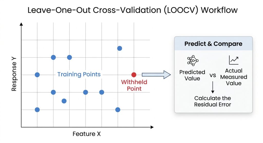
Leave-One-Out Cross-Validation evaluates a model by temporarily removing one observation, predicting its value from the remaining observations, and comparing that prediction with the actual measurement.

Suppose a dataset contains \(n\) sample locations:

\[ D=\{(s_i,z(s_i)):i=1,\ldots,n\} \]

where:

\(s_i\) represents the geographic coordinates of location \(i\).
\(z(s_i)\) is the observed value at that location.
\(n\) is the total number of observations.

For every observation, the procedure follows three steps:

Withhold: Remove one point from the data available to the interpolation model.
Predict: Estimate the value at the withheld point using the remaining observations.
Compare: Calculate the difference between the predicted value and the observed measurement.

The withheld point is restored, and the process repeats until every point has been predicted once. This produces \(n\) predictions and \(n\) corresponding errors.

Diagram illustrating the leave-one-out cross-validation workflow used to test spatial interpolation accuracy

2.2 Calculating prediction errors

Let \(\hat{z}_{-i}(s_i)\) represent the prediction for location \(i\) made without using that observation.

The cross-validation error is:

\[ e_i=\hat{z}_{-i}(s_i)-z(s_i) \]

This sign convention follows ArcGIS Pro documentation.

A positive residual means the model overpredicted the observed value.
A negative residual means the model underpredicted it.
A residual close to zero indicates a prediction close to the measurement.

For example, if the measured groundwater depth is 12.0 metres and the predicted depth is 13.2 metres, the error is:

\[ e_i=13.2-12.0=1.2\text{ m} \]

The prediction is 1.2 metres above the observed value.

The distinction between error and absolute error matters: positive and negative residuals can cancel when averaged, even when individual predictions are poor.

Important limitation: Some implementations estimate model parameters using all observations before withholding individual values. ArcGIS Pro documents this characteristic of its standard cross-validation procedure. For small datasets or influential outliers, it can introduce some information leakage. Fully nested LOOCV refits model parameters using only the training observations in each iteration, providing a stricter test.

3. Essential Geostatistical Error Metrics

Cross-validation produces individual residuals, but model comparison requires summary statistics. Five commonly used diagnostics are Mean Error (ME), Root Mean Square Error (RMSE), Mean Standardized Error, Root Mean Square Standardized Error (RMSS), and Average Standard Error.

Let \(e_i\) be the cross-validation error and \(\hat{\sigma}_i\) the estimated standard error of prediction at location \(i\).

3.1 Mean Error (ME): Measuring bias

Mean Error measures the average signed difference between predicted and measured values.

\[ ME=\frac{1}{n}\sum_{i=1}^{n}e_i \]

A desirable value is close to zero.

If ME is strongly positive, the model tends to overpredict. If it is strongly negative, the model tends to underpredict. However, a near-zero ME does not guarantee accurate predictions because large positive and negative errors can cancel one another.

Example: A model produces an ME of \(-0.15\) metres when predicting groundwater depth. This suggests a small average tendency to underpredict, although individual locations may still have substantial errors.

Interpret ME alongside RMSE rather than using it as a standalone accuracy measure.

3.2 Root Mean Square Error (RMSE): Measuring prediction accuracy

RMSE measures the magnitude of prediction errors while penalising large errors more heavily.

\[ RMSE=\sqrt{\frac{1}{n}\sum_{i=1}^{n}e_i^2} \]

RMSE is expressed in the same units as the measured variable. For example, a temperature interpolation model might have an RMSE of \(1.4^\circ\text{C}\).

When comparing models using the same observations and measurement units, lower RMSE generally indicates better predictive accuracy.

Unlike ME, RMSE cannot be reduced by positive and negative errors cancelling each other. Nevertheless, a few extreme residuals can disproportionately increase it.

Best practice: Use RMSE as a primary indicator when comparing IDW and Kriging, but inspect residual patterns and uncertainty diagnostics before selecting the final model.

3.3 Mean Standardized Error: Measuring standardized bias

In ArcGIS Pro, MSE refers to Mean Standardized Error, not the more commonly used statistical abbreviation for Mean Squared Error.

Each residual is divided by its estimated prediction standard error:

\[ SE_i^{*}=\frac{e_i}{\hat{\sigma}_i} \]

The mean standardized error is:

\[ MSE=\frac{1}{n}\sum_{i=1}^{n} \frac{e_i}{\hat{\sigma}_i} \]

The ideal value is approximately zero.

This statistic evaluates bias relative to the model’s own uncertainty estimates. It is particularly useful when comparing geostatistical models with different estimated prediction standard errors.

A value far from zero suggests systematic errors remain after accounting for predicted uncertainty. Interpretation also requires checking the model’s assumptions and whether standard errors are reliably estimated.

3.4 Root Mean Square Standardized Error (RMSS): Testing uncertainty calibration

RMSS measures the magnitude of standardized residuals:

\[ RMSS=\sqrt{\frac{1}{n}\sum_{i=1}^{n} \left(\frac{e_i}{\hat{\sigma}_i}\right)^2} \]

A well-calibrated model should generally have an RMSS close to 1.

RMSS result	Interpretation
Approximately 1	Estimated uncertainty is broadly consistent with observed errors.
Greater than 1	Prediction standard errors tend to be too small; uncertainty is underestimated.
Less than 1	Prediction standard errors tend to be too large; uncertainty is overestimated.

For example, RMSS = 1.8 suggests that observed cross-validation errors are larger relative to the estimated standard errors than expected under a well-calibrated model.

RMSS does not measure accuracy alone. A model can produce relatively good point predictions while still estimating uncertainty poorly.

3.5 Average Standard Error (ASE): Evaluating predicted uncertainty

Average Standard Error summarises the uncertainty estimates generated for cross-validation predictions.

In ArcGIS Pro, it is calculated as the root mean square of the individual prediction standard errors, rather than their simple arithmetic mean:

\[ ASE=\sqrt{\frac{1}{n}\sum_{i=1}^{n} \hat{\sigma}_i^2} \]

For a well-calibrated model, ASE should be reasonably close to RMSE. If ASE is substantially lower than RMSE, predicted uncertainty may be too optimistic. If ASE is considerably higher, the model may be overestimating uncertainty.

ASE should not simply be minimised in isolation. An unrealistically small uncertainty estimate is not evidence of a better model; the estimated uncertainty must also be consistent with observed errors.

How should the metrics be used together?

Metric	Main purpose	Preferred diagnostic
ME	Detect average bias	Close to 0
RMSE	Measure prediction error	Lower is better
Mean Standardized Error	Detect bias relative to uncertainty	Close to 0
RMSS	Assess uncertainty calibration	Close to 1
ASE	Summarise estimated prediction uncertainty	Similar to RMSE, with appropriate calibration

These values are complementary. RMSE assesses point prediction performance, while standardized errors and ASE evaluate whether the model’s uncertainty estimates are credible.

4. Comparing IDW and Kriging: Diagnostics and Model Behaviour

4.1 Inverse Distance Weighting

IDW is a deterministic interpolation method that estimates an unknown value using weighted observations. A common formulation is:

\[ \hat{z}(s_0)= \frac{\sum_{i=1}^{m}d_i^{-p}z(s_i)} {\sum_{i=1}^{m}d_i^{-p}} \]

where:

\(s_0\) is the prediction location.
\(d_i\) is the distance from sample \(i\) to \(s_0\).
\(p\) is the distance-power parameter.
\(m\) is the number of neighbouring points used.

Increasing \(p\) gives nearby observations greater influence. The chosen neighbourhood size and distance metric also affect predictions.

IDW is comparatively straightforward to configure, but it does not inherently provide the same statistical prediction standard errors as conventional kriging. In ArcGIS Pro, the documented cross-validation outputs for IDW include ME and RMSE, whereas the additional standard-error diagnostics are not available for that method.

Consequently, IDW should generally be compared with Kriging using common metrics such as ME and RMSE, rather than treating unavailable uncertainty statistics as zero.

4.2 Ordinary Kriging

Ordinary Kriging assumes an unknown but locally constant mean and uses spatial autocorrelation to determine prediction weights.

Unlike IDW, its weighting depends not only on distances to the sample points but also on the fitted semivariogram or covariance model.

A semivariogram describes how spatial variability changes with separation distance. Three parameters are especially important:

Nugget: Represents variation at very short distances, including measurement error and unresolved spatial variability.
Sill: The level at which the semivariogram levels off, representing the total variance under a bounded model.
Range: The distance at which the semivariogram reaches its sill and spatial autocorrelation becomes weak or negligible under that model.

The partial sill is the sill minus the nugget. Not every semivariogram model has a finite sill and range, so these definitions apply to bounded models.

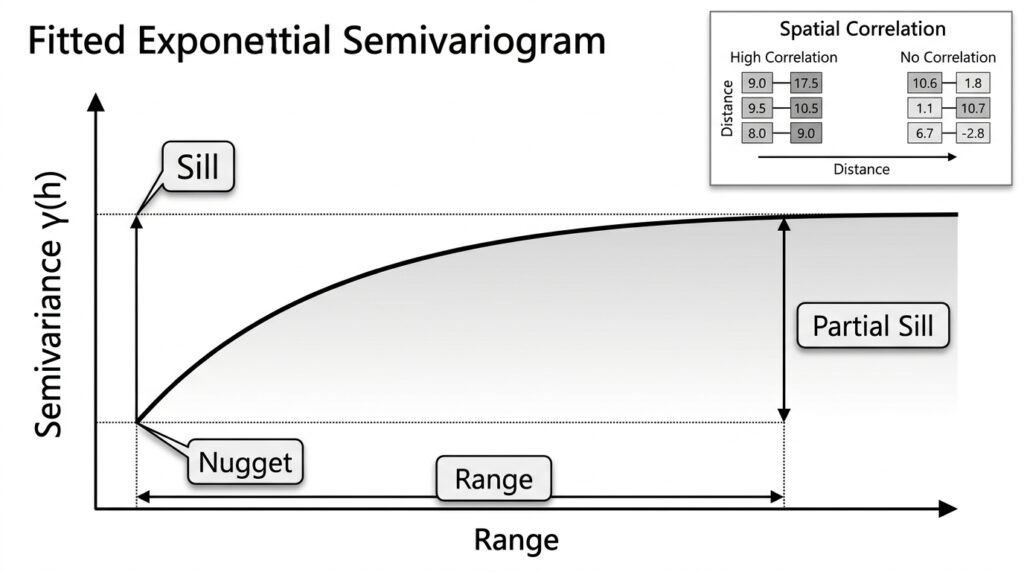
Labelled semivariogram diagram showing nugget, sill, and range for spatial interpolation accuracy assessment

These parameters influence both predicted values and prediction uncertainty. A larger nugget can indicate substantial local variability or measurement error; a longer range can imply that observations influence locations farther away. The sill affects the scale of modelled variability.

However, their effects on prediction standard errors depend on the combined model, sample geometry, neighbourhood configuration, and prediction location. A single parameter change does not guarantee lower uncertainty everywhere.

4.3 Universal Kriging

Universal Kriging accounts for a spatial trend, or drift, in the mean structure instead of assuming that the mean is locally constant.

For example, groundwater elevation may follow a regional gradient, while pollutant concentration may change systematically with distance from an industrial centre. Universal Kriging models the broad trend separately from the spatially correlated residual variation.

It can outperform Ordinary Kriging when the trend is real and modelled appropriately. If the trend is misspecified or unsupported by the data, however, it can introduce additional error.

IDW versus Kriging at a glance

Characteristic	IDW	Ordinary Kriging	Universal Kriging
Core approach	Distance-based weights	Spatial covariance and an unknown constant mean	Spatial covariance and a modelled trend
Key settings	Power, neighbours, search radius	Semivariogram, neighbourhood and mean assumptions	Semivariogram, trend structure and neighbourhood
Prediction standard errors	Not inherently supplied	Generally available	Generally available
Principal consideration	Sensitivity to point spacing and power	Quality of spatial autocorrelation model	Quality of both trend and autocorrelation models

The practical choice should be supported by cross-validation results and knowledge of the phenomenon being mapped, not by the complexity of the algorithm alone.

5. Practical Workflow in ArcGIS Pro and QGIS

The purpose of the workflow is to compare models using the same observations, the same measured attribute, and a consistent validation strategy.

5.1 Preparing your sample dataset

Before building either interpolation model:

Inspect the data. Confirm that the sampled attribute is numeric, the coordinates are valid, and missing or duplicate records are handled appropriately.
Choose a suitable coordinate reference system. For distance-based methods, use an appropriate projected coordinate system when working in a region where planar distances are suitable.
Examine the sampling pattern. Map sample locations and identify clusters, large gaps, edge effects, and unusual observations.
Check the attribute distribution. Calculate summary statistics and inspect histograms or boxplots for skewness and outliers.
Define the evaluation strategy. Use LOOCV for initial model comparison, and consider independent or spatially blocked validation when the intended use involves prediction in unsampled areas.

The IDW results can deteriorate when sample points are distributed unevenly, making a sampling-pattern inspection especially important.

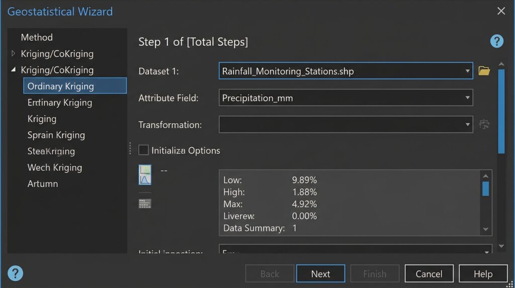
5.2 ArcGIS Pro: Cross-validation using Geostatistical Wizard

ArcGIS Pro provides a dedicated workflow for geostatistical interpolation and diagnostics through the Geostatistical Analyst extension.

[Image Suggestion: ArcGIS Pro Geostatistical Wizard showing the input point layer, selected interpolation attribute, and the available interpolation methods.]

Step 1: Add the data and select an attribute.

Load the point dataset into a map and open the Geostatistical Wizard. Select the field containing the variable to interpolate, such as nitrate concentration, soil pH, or groundwater depth.

Step 2: Build the IDW model.

Select IDW and configure its power parameter, search neighbourhood, and number of neighbours where applicable. Record the settings so that the model can be reproduced.

Step 3: Build the Kriging model.

Select Ordinary Kriging or Universal Kriging, depending on the structure of the data. Examine the empirical semivariogram, choose an appropriate theoretical model, and inspect the nugget, sill, and range.

For Universal Kriging, investigate whether a trend is justified by the sampling design and the process being modelled.

Step 4: Review cross-validation diagnostics.

Proceed to the final wizard page, where cross-validation statistics are available. Review ME and RMSE for both models. For Kriging, additionally inspect ASE, Mean Standardized Error, and RMSS where supported.

Compare results under consistent settings and retain the model parameters used in each run.

Step 5: Inspect cross-validation charts.

ArcGIS Pro provides a predicted-versus-measured scatter plot and additional diagnostics, including error and standardized-error plots.

ArcGIS Pro Geostatistical Wizard interface for analyzing spatial interpolation accuracy

Interpret the charts as follows:

Measured versus predicted: Points close to the 1:1 line indicate that predictions are close to observations.
Regression trend: A line close to the 1:1 reference suggests limited systematic scale and offset errors. A slope below or above 1 can reveal compression or exaggeration of the predicted range, depending on the axes.
Error versus measured values: Residuals should fluctuate around zero without strong systematic patterns. A trend may indicate bias or a smoothing effect.
Standardized-error plot: Patterns or unusually large standardized errors can indicate model inadequacy, local anomalies, or unreliable standard-error estimates.

Kriging commonly smooths extremes towards the central tendency. Therefore, underprediction of large measurements and overprediction of small measurements can occur even when overall accuracy is reasonable.

Step 6: Select and document the model.

Give preference to models that have lower RMSE, negligible bias, and credible uncertainty diagnostics. If two models perform similarly, favour the one with defensible assumptions, stable performance, and an appropriate spatial interpretation.

5.3 QGIS: Building a cross-validation workflow

QGIS provides an IDW interpolation algorithm through its Processing framework. Its standard IDW tool produces an interpolated raster, but that output alone is not a complete LOOCV assessment.

For QGIS, the validation process generally requires an automated iteration or an appropriate external validation tool.

Step 1: Prepare the points.

Load the sample layer, confirm the interpolated field, and check the coordinate system and units. Create a stable unique ID for each sample.

Step 2: Configure the interpolation model.

Open the Processing Toolbox and locate the IDW interpolation algorithm. Configure the input layer, attribute, power parameter where exposed, output extent, and raster cell size.

For Kriging, use a compatible installed Processing provider or geostatistical tool that supports the required kriging method. Confirm which prediction and uncertainty outputs it actually produces.

Step 3: Implement LOOCV.

For each sample point, exclude that point from the training dataset, fit or configure the model using the remaining observations, and predict at the withheld coordinate. Store the point ID, measured value, predicted value, and residual in a table.

Repeat for every point. Python with PyQGIS or another suitable geospatial library can automate this process. When testing fitted Kriging models, refit the trend and spatial-correlation parameters within each iteration for a strict LOOCV implementation.

Step 4: Calculate the error statistics.

Using the resulting table, calculate ME and RMSE for both methods. If the Kriging implementation provides prediction standard errors, calculate Mean Standardized Error, RMSS, and ASE as well.

Step 5: Examine error patterns.

Join the residual table back to the sample locations and map the errors. Spatially concentrated positive or negative residuals may reveal model bias, missing trend structure, or environmental boundaries that the interpolation fails to represent.

Important: QGIS Processing providers can differ in their available algorithms and parameters. Record the provider, software version, model settings, and validation method so another analyst can reproduce the results.

6. Common Pitfalls and Best Practices

Even correctly calculated geostatistical error metrics can give a misleading impression if the validation design or underlying data is inappropriate.

6.1 Clustered and unevenly distributed samples

Dense clusters contain more nearby observations than sparsely sampled regions. A model may perform well around clusters but poorly in areas with limited coverage. Because ordinary LOOCV may leave nearby samples available to predict a withheld point, it can underestimate errors in genuinely unsampled regions.

Best practice: Map sample density, examine residuals geographically, and consider spatially blocked validation when predicting beyond well-sampled areas.

6.2 Skewed distributions and outliers

Highly skewed measurements, such as pollutant concentrations, can produce large residuals that dominate RMSE. Outliers may represent measurement errors, genuine hotspots, or local processes that the model cannot capture.

Best practice: Investigate extreme observations before removing them. Consider transformations where statistically and scientifically justified, and assess whether a few locations dominate the error statistics.

6.3 Anisotropy and spatial trends

Anisotropy occurs when spatial continuity changes with direction. For example, groundwater levels may be more strongly correlated along a geological formation than across it. A directional mismatch between the semivariogram and the underlying process can weaken predictions.

Best practice: Explore directional spatial dependence and investigate whether anisotropic semivariogram models or trend-aware interpolation are justified.

6.4 Low RMSE does not guarantee a realistic surface

Cross-validation assesses predictions at sampled locations; it does not prove that every unsampled cell is physically plausible. An interpolation can achieve a low RMSE while producing unrealistic gradients, ignoring barriers, smoothing important extremes, or extrapolating beyond the supported data range.

Best practice: Combine geostatistical error metrics with field knowledge, spatial diagnostics, plausible value ranges, and independent validation when available. Cross-validation is evidence of predictive performance, not proof of physical realism.

7. Conclusion: Turning Interpolation into Evidence-Based Analysis

Cross-validation provides a quantitative foundation for comparing IDW and Kriging. It allows GIS analysts to test predictions against known measurements, diagnose systematic errors, and assess whether estimated uncertainty is consistent with observed performance.

RMSE is useful for comparing prediction accuracy, ME reveals average bias, and Kriging’s standardized-error statistics help evaluate uncertainty calibration. However, none of these metrics should be interpreted in isolation.

Before finalising an interpolation model, use this checklist:

Verify sample quality, coordinate systems, and the spatial distribution of observations.
Apply a consistent LOOCV procedure to IDW and Kriging.
Compare ME and RMSE using the same observations and measurement units.
Where available, inspect ASE, Mean Standardized Error, and RMSS.
Examine predicted-versus-measured plots and map residual patterns.
Evaluate clustering, outliers, anisotropy, and possible spatial trends.
Use independent or spatially blocked validation when the intended prediction task requires it.
Document model parameters, software versions, assumptions, and limitations.

Ultimately, the best interpolation model is not necessarily the one that produces the smoothest map or the lowest RMSE. It is the model that combines reliable predictive performance, defensible spatial assumptions, appropriately calibrated uncertainty, and a meaningful interpretation of the geographic phenomenon.