
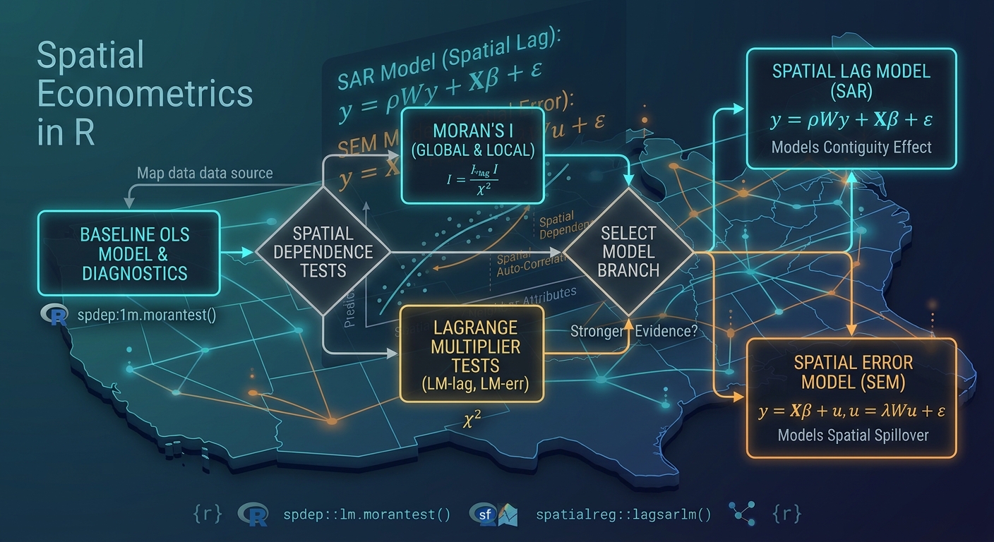
Spatial Regression with R: Fitting Spatial Lag and Spatial Error Models in spdep
Introduction
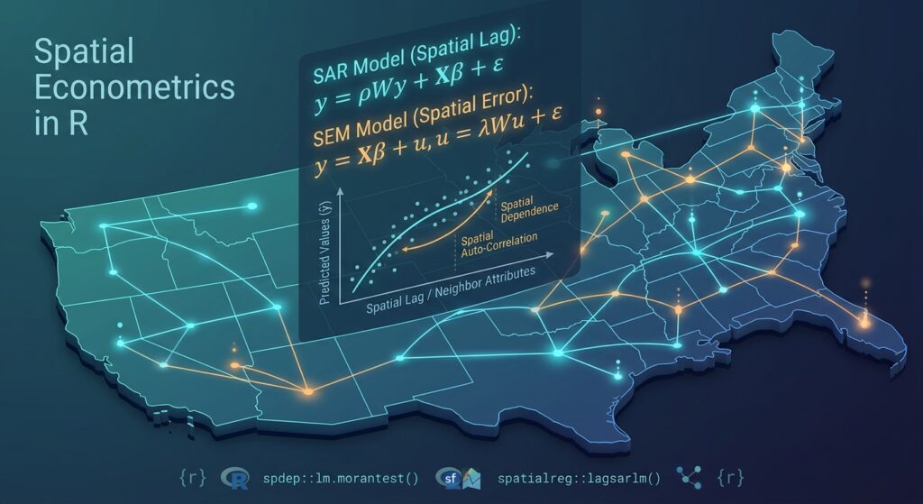
When performing spatial regression with R spdep, Ordinary Least Squares (OLS) is often the natural starting point for regression analysis. Ordinary Least Squares (OLS) is often the natural starting point for regression analysis. In a conventional linear model, we assume that observations are sufficiently independent that the error terms do not exhibit systematic spatial relationships.
That assumption can be problematic when the observations are geographic units such as counties, census tracts, wards, districts, or administrative polygons.
For example, suppose we model household income across neighboring counties. Economic conditions in one county may influence neighboring counties, while similar counties may also share unobserved regional characteristics. Consequently, observations that are geographically close may not be statistically independent.
A conventional OLS model can be written as:
\[ y = X\beta + \epsilon \]
where:
- \(y\) = dependent variable
- \(X\) = explanatory variables
- \(\beta\) = regression coefficients
- \(\epsilon\) = error term
When spatial dependence exists, the error structure may violate the assumptions underlying conventional OLS inference. Standard errors can become unreliable, making significance tests and p-values misleading.
Spatial econometrics addresses this problem by explicitly incorporating relationships between neighboring observations.
Two fundamental models are:
Spatial Lag Model (SAR):
\[ y = \rho Wy + X\beta + \epsilon \]
where \(\rho\) measures dependence between the dependent variable and neighboring observations.
Spatial Error Model (SEM):
\[ y = X\beta + u \]
with
\[ u = \lambda Wu + \epsilon \]
where \(\lambda\) represents spatial dependence in the error process.
In R, packages such as spdep and spatialreg provide tools for constructing spatial weights, diagnosing spatial dependence, and estimating these models.
1. Prerequisites
We will use four main R packages:
sf— reading and manipulating spatial vector dataspdep— spatial weights and spatial dependence diagnosticsspatialreg— spatial regression modelstmap— mapping and visual inspection
Install them if necessary:
# Install packages once if they are not already installed
install.packages(c(
  "sf",
  "spdep",
  "spatialreg",
  "tmap"
))
Load the packages:
# Load required libraries
library(sf)
library(spdep)
library(spatialreg)
library(tmap)
A useful distinction is that spdep is particularly important for spatial-neighbor structures and diagnostics, while spatialreg contains functions for estimating spatial regression models such as lagsarlm() and errorsarlm().
2. Load Spatial Polygon Data
For this tutorial, assume you have a polygon dataset containing geographic units and socioeconomic variables.
For example:
income— average household incomeunemployment— unemployment rateeducation— percentage of adults with higher educationpopulation_density— population per square kilometer
Suppose the dataset is stored as:
data/counties.shpRead it with sf:
# Read polygon data
counties <- st_read("data/counties.shp")

# Inspect the dataset
print(counties)

# Display attribute names
names(counties)

# Check the coordinate reference system
st_crs(counties)
You should verify that the variables required for your regression actually exist:
# Examine the first few observations
head(counties)

# Check the structure of the attribute table
str(counties)
Visualize the dependent variable
Before modeling, map the dependent variable.
# Basic thematic map
tm_shape(counties) +
  tm_polygons(
    col = "income",
    title = "Average Income"
  )
This is not merely cosmetic. Mapping the dependent variable can reveal broad geographic patterns that may later manifest as spatial autocorrelation.
3. Run a Baseline OLS Regression
Start with the conventional model before introducing spatial econometrics.
Suppose we want to explain income using unemployment, education, and population density.
# Fit conventional OLS model
ols_model <- lm(
  income ~ unemployment +
    education +
    population_density,
  data = counties
)

# Display regression results
summary(ols_model)
The output will contain coefficients such as:
Coefficients:

                     Estimate   Std. Error   t value   Pr(>|t|)
(Intercept)            ...
unemployment           ...
education              ...
population_density     ...
The coefficient estimates describe the association between each explanatory variable and income, holding the other variables constant.
For example, if the coefficient for education is positive, the model estimates that higher education levels are associated with higher income, conditional on the other predictors.
However, these coefficients should not yet be interpreted as proof that OLS is appropriate.
The next question is:
Are the OLS residuals spatially independent?
4. Build a Spatial Weights Matrix
Spatial econometric models need a formal definition of which observations are considered neighbors.
For polygon data, two common approaches are:
- Queen contiguity — polygons sharing either an edge or a vertex are neighbors.
- Rook contiguity — polygons must share an edge to be neighbors.
The resulting neighbor structure is represented using a spatial weights matrix.
4.1 Queen Contiguity
Use poly2nb():
# Create Queen-contiguity neighbors
queen_nb <- poly2nb(
  counties,
  queen = TRUE
)

# Inspect the neighbor object
queen_nb
You can inspect the neighbors of individual polygons:
# Neighbors of the first five polygons
queen_nb[1:5]
For example, if polygon 1 returns:
1: 2 5 8then polygons 2, 5, and 8 are considered neighbors of polygon 1.
4.2 Rook Contiguity
Create a Rook-based neighbor structure with:
# Create Rook-contiguity neighbors
rook_nb <- poly2nb(
  counties,
  queen = FALSE
)

# Inspect the neighbor structure
rook_nb
The difference is important.
Imagine two polygons touching only at one corner:
+-----+
|  A  |
+-----+
      +
      | B |
      +
Under Queen contiguity, they can be neighbors.
Under Rook contiguity, they are not neighbors because they do not share an edge.
5. Convert Neighbors to Spatial Weights
poly2nb() creates a neighbor list, but spatial regression functions need a spatial weights object.
Use nb2listw():
# Convert Queen neighbors to row-standardized spatial weights
queen_listw <- nb2listw(
  queen_nb,
  style = "W"
)

# Inspect the weights object
queen_listw
The "W" style creates row-standardized weights.
For an observation with four neighbors, for example, each neighbor may receive a weight of:
\[ \frac{1}{4}=0.25 \]
This means the spatial lag can be interpreted approximately as a weighted average of neighboring observations.
You can create Rook weights in exactly the same way:
# Convert Rook neighbors to spatial weights
rook_listw <- nb2listw(
  rook_nb,
  style = "W"
)
For the rest of this tutorial, we will use the Queen-contiguity weights.
6. Check the Spatial Structure
It is useful to visualize the neighbor relationships.
# Obtain polygon centroids
centroids <- st_centroid(counties)

# Convert centroids to coordinates
coords <- st_coordinates(centroids)

# Plot polygons
plot(st_geometry(counties))

# Draw Queen neighbor links
plot(
  queen_nb,
  coords,
  add = TRUE,
  col = "red"
)
You should see lines connecting neighboring polygons.
This provides an important sanity check.
A spatial weights matrix is not automatically correct simply because poly2nb() successfully generated one. Your definition of “neighbor” should make substantive sense for the geographic process being modeled.
7. Test OLS Residuals for Spatial Autocorrelation
Now extract the OLS residuals:
# Extract OLS residuals
ols_residuals <- residuals(ols_model)
Use Moran’s I to test whether the residuals exhibit spatial autocorrelation:
# Moran's I test on OLS residuals
moran.test(
  ols_residuals,
  queen_listw
)
A typical result contains:
Moran I statistic
Expectation
Variance
p-value
The null hypothesis is approximately:
\[ H_0: I = E(I) \]
meaning that the residuals do not exhibit spatial autocorrelation under the specified spatial structure.
If the test produces a small p-value, there is evidence that the OLS residuals are spatially autocorrelated.
For example:
Moran I statistic = 0.31
p-value = 0.002
would provide evidence against spatial independence.
Why this matters
Suppose neighboring counties consistently have similar unexplained income values.
OLS does not explicitly model that geographic relationship.
The resulting inference may therefore underestimate or otherwise misrepresent uncertainty.
This is where spatial regression becomes useful.
8. Run Lagrange Multiplier Diagnostics
Moran’s I tells us that spatial autocorrelation exists, but we also want to investigate what type of spatial model may be appropriate.
The classic approach is to use Lagrange Multiplier (LM) diagnostics.
Depending on your installed spdep version, you may encounter the older lm.LMtests() interface or the newer lm.RStests() interface. For compatibility with workflows that specifically use lm.LMtests(), the following code illustrates the requested approach.
# Run Lagrange Multiplier diagnostics
lm_tests <- lm.LMtests(
  ols_model,
  queen_listw,
  test = "all"
)

# Display results
lm_tests
The diagnostics may include tests associated with:
- spatial lag dependence
- spatial error dependence
- robust spatial lag dependence
- robust spatial error dependence
Conceptually, these tests help answer:
Is the spatial dependence primarily associated with the dependent variable itself, or with the error process?
Important version note
In newer versions of spdep, some users may see a deprecation warning for lm.LMtests().
The modern equivalent is:
# Modern spatial regression diagnostics
lm.RStests(
  ols_model,
  queen_listw,
  test = "all"
)
If your installed version recommends lm.RStests(), use that function rather than treating the warning as a modeling error.
9. Understanding the Spatial Lag Model
The Spatial Lag Model, also called the Spatial Autoregressive Model (SAR), introduces the spatially lagged dependent variable:
\[ y = \rho Wy + X\beta + \epsilon \]
Here:
- \(y\) = dependent variable
- \(Wy\) = spatial lag of the dependent variable
- \(X\) = explanatory variables
- \(\beta\) = regression coefficients
- \(\rho\) = spatial autoregressive parameter
- \(\epsilon\) = random error
The term \(Wy\) represents neighboring values of the dependent variable.
For our income example:
\[ Wy \]
can be interpreted as a spatially weighted measure of neighboring counties’ income.
10. Fit the spatial Lag Model in R using Spatial Regression with R spdep
Use lagsarlm() from spatialreg:
# Fit Spatial Lag Model
lag_model <- lagsarlm(
  income ~ unemployment +
    education +
    population_density,
  data = counties,
  listw = queen_listw
)

# Display model results
summary(lag_model)
The output contains the ordinary regression coefficients plus the spatial autoregressive parameter:
Rho: ...10.1 Interpreting \(\rho\)
The parameter \(\rho\) measures spatial dependence in the dependent variable.
Suppose you obtain:
rho = 0.42A positive value indicates positive spatial dependence: higher values of the dependent variable in neighboring areas are associated with higher values in the focal area, after accounting for the explanatory variables.
A value near zero indicates relatively weak spatial lag dependence.
A negative value indicates negative spatial dependence.
However, do not interpret \(\rho\) as an ordinary regression slope.
The model contains feedback because each area’s outcome is related to neighboring outcomes, while those neighbors are themselves related to other areas.
Therefore, interpreting SAR models through the ordinary “one-unit increase in X produces a β-unit change in Y” framework can be misleading.
11. Calculate Spatial Lag Impacts
For a spatial lag model, coefficient interpretation is more complicated because of spatial feedback.
spatialreg provides impact calculations.
# Calculate direct, indirect, and total impacts
lag_impacts <- impacts(
  lag_model,
  listw = queen_listw,
  R = 1000
)

# Display impacts
summary(lag_impacts)
The results generally distinguish between:
- Direct impacts — effects within the focal observation
- Indirect impacts — spillover effects across neighboring observations
- Total impacts — combined direct and indirect effects
This is often more informative than interpreting the raw SAR coefficient alone.
12. Fit the Spatial Error Model
The Spatial Error Model (SEM) assumes that spatial dependence occurs in the error process rather than directly through the dependent variable.
The model can be expressed as:
\[ y=X\beta+u \]
where:
\[ u=\lambda Wu+\epsilon \]
The parameter \(\lambda\) measures spatial dependence among the model errors.
This is useful when omitted regional factors, measurement issues, institutional effects, environmental conditions, or other unobserved processes are spatially clustered.
13. Estimate the Spatial Error Model in R
Use errorsarlm():
# Fit Spatial Error Model
error_model <- errorsarlm(
  income ~ unemployment +
    education +
    population_density,
  data = counties,
  listw = queen_listw
)

# Display model results
summary(error_model)
The output includes:
Lambda: ...13.1 Interpreting \(\lambda\)
Suppose:
lambda = 0.55A positive \(\lambda\) suggests that unexplained components of income are spatially correlated.
In practical terms, neighboring counties may share unobserved characteristics that the explanatory variables do not capture.
For example, nearby areas could share:
- regional economic policies
- infrastructure systems
- labor markets
- environmental conditions
- historical institutions
- unmeasured socioeconomic characteristics
Unlike the SAR model, the SEM does not directly introduce neighboring values of income into the structural equation.
Instead, spatial dependence is modeled through the disturbance process.
14. Compare OLS, Spatial Lag, and Spatial Error Models
At this point we have three models:
# OLS
ols_model

# Spatial Lag
lag_model

# Spatial Error
error_model
A simple comparison can be created with:
# Compare AIC values
AIC(
  ols_model,
  lag_model,
  error_model
)
You can also compare log-likelihood values:
# Compare log-likelihoods
logLik(ols_model)
logLik(lag_model)
logLik(error_model)
A convenient summary table is:
# Create a simple model comparison table
model_comparison <- data.frame(
  Model = c(
    "OLS",
    "Spatial Lag",
    "Spatial Error"
  ),
  AIC = c(
    AIC(ols_model),
    AIC(lag_model),
    AIC(error_model)
  ),
  LogLik = c(
    as.numeric(logLik(ols_model)),
    as.numeric(logLik(lag_model)),
    as.numeric(logLik(error_model))
  )
)

# Display comparison
model_comparison
You might obtain a table resembling:
           Model      AIC    LogLik
1           OLS   1250.4   -620.2
2   Spatial Lag   1218.7   -602.4
3 Spatial Error   1223.1   -604.6
These numbers are illustrative; your actual results will depend on your dataset.
14.1 Interpreting AIC
The Akaike Information Criterion balances model fit against model complexity.
Generally:
Lower AIC indicates a better trade-off between fit and complexity among the models being compared.
Therefore, if the Spatial Lag Model has a substantially lower AIC than OLS, that provides evidence that explicitly modeling spatial dependence improves the model according to AIC.
But AIC should not be used in isolation.
You should also consider:
- spatial diagnostics
- theoretical justification
- coefficient stability
- residual spatial autocorrelation
- model assumptions
- the spatial process being studied
14.2 Interpreting Log-Likelihood
The log-likelihood measures how well the model explains the observed data under its assumed probability structure.
For models estimated on the same dependent variable and observations, a higher log-likelihood generally indicates better fit.
For example:
OLS              -620.2
Spatial Lag      -602.4
Spatial Error    -604.6
Both spatial models would have improved likelihood relative to OLS in this illustrative example.
However, log-likelihood alone does not penalize additional model complexity. That is one reason AIC is useful for comparison.
15. A Complete Reproducible Workflow
The entire workflow can be condensed into the following script.
# ============================================================
# SPATIAL REGRESSION WITH R
# OLS vs Spatial Lag vs Spatial Error
# ============================================================

# ------------------------------------------------------------
# 1. Load packages
# ------------------------------------------------------------

library(sf)
library(spdep)
library(spatialreg)
library(tmap)


# ------------------------------------------------------------
# 2. Load spatial polygon data
# ------------------------------------------------------------

counties <- st_read("data/counties.shp")

# Inspect data
print(counties)
names(counties)


# ------------------------------------------------------------
# 3. Baseline OLS regression
# ------------------------------------------------------------

ols_model <- lm(
  income ~ unemployment +
    education +
    population_density,
  data = counties
)

summary(ols_model)


# ------------------------------------------------------------
# 4. Build Queen spatial neighbors
# ------------------------------------------------------------

queen_nb <- poly2nb(
  counties,
  queen = TRUE
)


# ------------------------------------------------------------
# 5. Convert neighbors to spatial weights
# ------------------------------------------------------------

queen_listw <- nb2listw(
  queen_nb,
  style = "W"
)


# ------------------------------------------------------------
# 6. Check OLS residual spatial autocorrelation
# ------------------------------------------------------------

ols_residuals <- residuals(ols_model)

moran.test(
  ols_residuals,
  queen_listw
)


# ------------------------------------------------------------
# 7. Lagrange Multiplier diagnostics
# ------------------------------------------------------------

# Older/common interface
lm.LMtests(
  ols_model,
  queen_listw,
  test = "all"
)

# Newer spdep versions may use:
lm.RStests(
  ols_model,
  queen_listw,
  test = "all"
)


# ------------------------------------------------------------
# 8. Spatial Lag Model
# ------------------------------------------------------------

lag_model <- lagsarlm(
  income ~ unemployment +
    education +
    population_density,
  data = counties,
  listw = queen_listw
)

summary(lag_model)


# ------------------------------------------------------------
# 9. Spatial Error Model
# ------------------------------------------------------------

error_model <- errorsarlm(
  income ~ unemployment +
    education +
    population_density,
  data = counties,
  listw = queen_listw
)

summary(error_model)


# ------------------------------------------------------------
# 10. Compare model performance
# ------------------------------------------------------------

model_comparison <- data.frame(
  Model = c(
    "OLS",
    "Spatial Lag",
    "Spatial Error"
  ),

  AIC = c(
    AIC(ols_model),
    AIC(lag_model),
    AIC(error_model)
  ),

  LogLik = c(
    as.numeric(logLik(ols_model)),
    as.numeric(logLik(lag_model)),
    as.numeric(logLik(error_model))
  )
)

print(model_comparison)


# ------------------------------------------------------------
# 11. Spatial impacts for SAR model
# ------------------------------------------------------------

lag_impacts <- impacts(
  lag_model,
  listw = queen_listw,
  R = 1000
)

summary(lag_impacts)
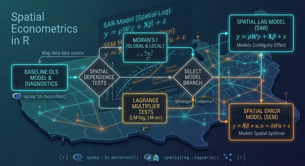
16. A Practical Decision Framework
The workflow should not simply be:
OLS → SAR → SEM → choose whichever has the lowest AIC.
Instead, think of the process as a sequence of statistical questions.
| Stage | Question | R function |
|---|---|---|
| 1 | What is the baseline relationship? | lm() |
| 2 | Are residuals spatially autocorrelated? | moran.test() |
| 3 | What type of spatial dependence is suggested? | lm.LMtests() / lm.RStests() |
| 4 | Is dependence associated with neighboring outcomes? | lagsarlm() |
| 5 | Is dependence primarily in unobserved errors? | errorsarlm() |
| 6 | Which model provides better fit? | AIC(), logLik() |
| 7 | What are the SAR spillover effects? | impacts() |
This distinction is important because spatial autocorrelation is a property of the data-generating process, not merely a nuisance to eliminate.
17. Common Problems and Troubleshooting
Problem 1: Invalid geometries
Spatial neighbor construction can fail or behave unexpectedly when polygons contain invalid geometries.
Check them with:
# Check geometry validity
sum(!st_is_valid(counties))
Repair invalid geometries:
# Repair invalid geometries
counties <- st_make_valid(counties)
Then recreate the neighbor structure.
Problem 2: Islands with no neighbors
Some polygon datasets contain isolated geographic units.
Check:
# Identify polygons without neighbors
which(card(queen_nb) == 0)
If an observation has no neighbors, nb2listw() may require special handling.
For example:
queen_listw <- nb2listw(
  queen_nb,
  style = "W",
  zero.policy = TRUE
)
Use this deliberately rather than automatically. A zero-neighbor observation may indicate a genuine geographic characteristic or a problem with the dataset.
Problem 3: Coordinate reference system
For polygon contiguity, the geographic CRS itself is not necessarily a problem because contiguity is based on polygon topology.
However, if you later perform distance-based analysis, projections become much more important.
Inspect your CRS:
st_crs(counties)For distance-based spatial weights, consider an appropriate projected CRS.
18. Queen vs Rook: Which Should You Use?
There is no universal winner.
Use Queen contiguity when touching at a corner represents meaningful interaction.
Use Rook contiguity when sharing a boundary is a more defensible definition of spatial interaction.
You can even test the sensitivity of your conclusions to the choice of weights:
# Queen weights
queen_nb <- poly2nb(counties, queen = TRUE)

queen_listw <- nb2listw(
  queen_nb,
  style = "W"
)

# Rook weights
rook_nb <- poly2nb(counties, queen = FALSE)

rook_listw <- nb2listw(
  rook_nb,
  style = "W"
)
Then estimate the same model using both:
# Queen-based SAR
sar_queen <- lagsarlm(
  income ~ unemployment +
    education +
    population_density,
  data = counties,
  listw = queen_listw
)

# Rook-based SAR
sar_rook <- lagsarlm(
  income ~ unemployment +
    education +
    population_density,
  data = counties,
  listw = rook_listw
)
If substantive conclusions change dramatically depending on the weights matrix, that sensitivity should be discussed rather than hidden.
19. What You Should Report in an Applied Study
For a thesis, research paper, or GIS analysis, reporting only the regression coefficients is usually insufficient.
Document:
- Spatial units used
- Dependent and independent variables
- OLS specification
- Spatial weights definition
- Queen or Rook contiguity
- Weight standardization method
- Moran’s I results
- LM diagnostic results
- SAR/SEM parameter estimates
- AIC and log-likelihood
- Residual diagnostics
- Direct, indirect, and total impacts for SAR models where appropriate
For example, your methodology might state that polygon neighbors were defined using Queen contiguity and converted to row-standardized weights before testing OLS residuals for spatial autocorrelation and estimating alternative spatial regression specifications.
Summary
A conventional OLS regression assumes that the unexplained component of observations is appropriately modeled without spatial dependence. Geographic data frequently violate this assumption because neighboring areas can influence one another or share unobserved characteristics.
The spdep and spatialreg ecosystem provides a practical workflow for addressing this problem.
The core process is:
Spatial polygons
      ↓
      sf
      ↓
Baseline OLS
      ↓
poly2nb()
      ↓
nb2listw()
      ↓
Moran's I
      ↓
LM diagnostics
      ↓
 ┌───────────────┐
 │               │
SAR             SEM
 │               │
lagsarlm()      errorsarlm()
 │               │
 └───────┬───────┘
         ↓
 AIC + Log-Likelihood
         ↓
Model interpretation
The key lesson is that spatial regression is not simply OLS with a different function. You first need to establish how observations are connected geographically, diagnose whether spatial dependence exists, identify the likely form of that dependence, and then interpret the resulting spatial parameters appropriately.
For a Spatial Lag Model, focus on \(\rho\) and the resulting direct, indirect, and total impacts. For a Spatial Error Model, focus on \(\lambda\) and the evidence that spatial dependence remains in the disturbance process.
Ultimately, a good spatial regression analysis combines statistical diagnostics, geographic reasoning, and model comparison rather than selecting a model solely because it produces a lower AIC.