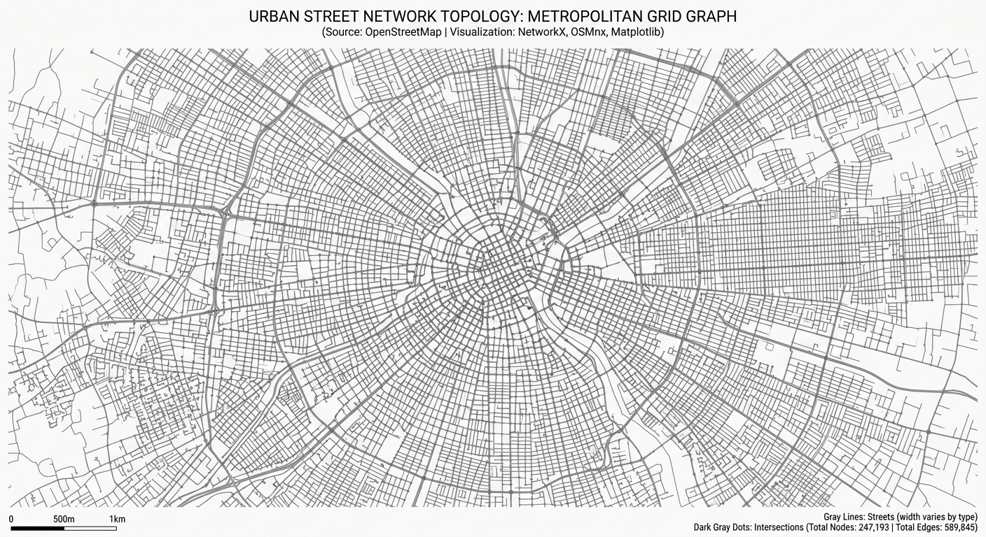
Analyzing Spatial Networks in Python with OSMnx and NetworkX

Introduction

Urban street networks shape how people move through cities and access essential services. The arrangement of intersections, road segments, and pedestrian pathways influences travel distance, route choice, and accessibility to schools, hospitals, public transport, and employment.

For urban planners and geospatial analysts, understanding these relationships requires more than measuring distances between points on a map. Two neighbourhoods may be equally close to a hospital in straight-line distance but have very different levels of accessibility because of disconnected streets, restricted crossings, or indirect routes.

OSMnx makes this analysis possible directly in Python. It retrieves street-network data from OpenStreetMap, constructs graph representations, calculates network statistics, and supports spatial visualization. NetworkX complements OSMnx with algorithms for graph connectivity, centrality, and shortest-path routing.

Together, these libraries provide a reproducible framework for OSMnx NetworkX Python spatial network analysis, allowing analysts to move from raw street data to quantitative urban insights without manually digitizing road networks.

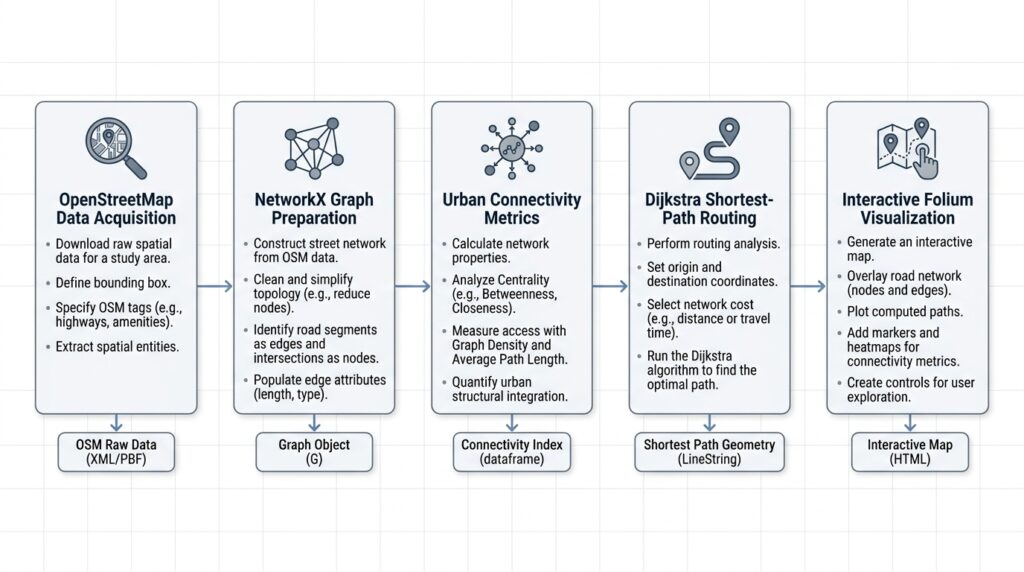
This tutorial develops a practical workflow using a pedestrian street network. You will download the data, prepare the graph, calculate urban connectivity metrics, find a shortest route using Dijkstra’s algorithm, and create an interactive map of the results.

1. Set up the Python environment

1.1 Install the required libraries

Install the following packages in your Python environment:

pip install osmnx networkx geopandas pandas matplotlib folium

The workflow uses these libraries for different tasks:

Library	Purpose
OSMnx	Download, project, analyze, and visualize street networks
NetworkX	Calculate graph metrics and shortest paths
GeoPandas	Store and export spatial features
pandas	Organize network statistics and tabular results
Matplotlib	Produce static network maps
Folium	Generate interactive HTML maps

This tutorial uses the OSMnx 2.x API. If you have an older installation, check the documentation for differences in function names and arguments.

1.2 Import the libraries

Create a Python script named urban_network_analysis.py.

from pathlib import Path

import osmnx as ox
import networkx as nx
import geopandas as gpd
import pandas as pd
import matplotlib.pyplot as plt
import folium

# Create a directory for the outputs.
OUTPUT_DIR = Path("urban_network_outputs")
OUTPUT_DIR.mkdir(parents=True, exist_ok=True)

# Enable local caching of downloaded responses.
ox.settings.use_cache = True

print("OSMnx version:", ox.__version__)
print("NetworkX version:", nx.__version__)
print("Output directory:", OUTPUT_DIR.resolve())

Caching can reduce repeated network requests when rerunning the script. The initial download still requires an internet connection.

2. Download a street network from OpenStreetMap

The first step is selecting a network that reflects the type of movement being studied. A pedestrian network differs from a vehicle network because some roads, paths, and access restrictions apply differently to each mode.

2.1 Download a network using graph_from_place()

OSMnx’s graph_from_place() function geocodes a named location and constructs a graph from the mapped street features within its boundary.

For this example, use Nairobi, Kenya.

# Define the study area.
PLACE = "Nairobi, Kenya"

# Download the pedestrian street network.
G = ox.graph.graph_from_place(
    PLACE,
    network_type="walk",
    simplify=True,
    retain_all=False,
)

# Report the network dimensions.
print("Study area:", PLACE)
print("Number of nodes:", G.number_of_nodes())
print("Number of edges:", G.number_of_edges())

# Confirm the graph representation.
print("Graph type:", type(G).__name__)

The main parameters control how the network is constructed:

• network_type="walk" requests a network intended for pedestrian analysis.
• simplify=True removes unnecessary intermediate nodes while preserving important junctions and endpoints.
• retain_all=False keeps the largest weakly connected component rather than every disconnected component.

For vehicle routing, use network_type="drive". Cycling studies can use network_type="bike".

Important: Selecting a network type does not guarantee complete pedestrian or road coverage. OpenStreetMap completeness varies by location, and the available paths depend on how features have been mapped and tagged.

Keeping only the largest connected component can also remove smaller but potentially important networks. Use retain_all=True when isolated paths or disconnected urban areas are part of the research question.

2.2 Download a network using a bounding box

A bounding box is useful when your analysis focuses on a particular neighbourhood or corridor rather than an entire administrative area.

# Define the bounding box in longitude and latitude.
# Order: west, south, east, north.
bbox = (
    36.78,   # West
    -1.31,   # South
    36.88,   # East
    -1.24,   # North
)

# Retrieve the pedestrian network within the bounding box.
G = ox.graph.graph_from_bbox(
    bbox=bbox,
    network_type="walk",
    simplify=True,
    retain_all=False,
)

print("Nodes:", G.number_of_nodes())
print("Edges:", G.number_of_edges())

The coordinates must be supplied in the order expected by the current OSMnx API: west, south, east, north. They represent longitude and latitude, not projected metres.

Use either the place-based or bounding-box approach for the main workflow. If you use the bounding-box version, remember that the rectangular extent may include areas outside the administrative boundary you ultimately want to study.

2.3 Save the downloaded graph

Downloading the same network repeatedly wastes time and may produce different results as OpenStreetMap changes. Save the graph for reuse.

# Save the network in GraphML format.
graph_path = OUTPUT_DIR / "urban_street_network.graphml"

ox.io.save_graphml(
    G,
    filepath=graph_path,
)

print("Graph saved:", graph_path)

Load the saved graph in a later session:

# Reload the saved graph without downloading it again.
G = ox.io.load_graphml(graph_path)

print("Reloaded nodes:", G.number_of_nodes())
print("Reloaded edges:", G.number_of_edges())

GraphML preserves graph topology and associated attributes, making it suitable for repeatable network-analysis projects.

3. Prepare and project the graph

Before measuring distances or densities, inspect the graph’s coordinate reference system and structure. Network data downloaded from OpenStreetMap typically uses geographic coordinates, which are appropriate for location-based mapping but not ideal for planar distance calculations.

3.1 Project the network into a metric coordinate system

# Project the graph into a suitable local projected CRS.
G_proj = ox.projection.project_graph(G)

# Convert graph nodes and edges into spatial tables.
nodes_gdf, edges_gdf = ox.convert.graph_to_gdfs(G_proj)

# Inspect the coordinate reference system.
print("Projected CRS:", G_proj.graph["crs"])

# Inspect the first few records.
print(nodes_gdf.head())
print(edges_gdf.head())

OSMnx automatically selects a suitable local projection when one is not specified. For many urban studies, this provides coordinates in metres, making it easier to calculate lengths and areas.

The node GeoDataFrame contains point geometries and node attributes. The edge GeoDataFrame contains street-segment geometries and attributes such as length.

3.2 Understand the graph structure

OSMnx represents street networks as directed multigraphs.

• Nodes represent network locations, including intersections and endpoints.
• Edges represent connections between nodes.
• Directed edges preserve permitted travel directions.
• Parallel edges allow multiple connections between the same pair of nodes.
• Simplified edges can represent complete street segments rather than individual geometry vertices.

These details affect how connectivity metrics should be interpreted. A two-way road may be represented by reciprocal directed edges, so counting directed edges is not equivalent to counting physical streets.

For shortest-path routing, retain the directed graph when one-way restrictions matter. For physical street-connectivity summaries, use an appropriate street-counting method rather than assuming that graph degree equals the number of roads at an intersection.

3.3 Export the network for GIS inspection

# Export the projected nodes and edges to GeoPackage.
nodes_gdf.to_file(
    OUTPUT_DIR / "street_nodes.gpkg",
    driver="GPKG",
)

edges_gdf.to_file(
    OUTPUT_DIR / "street_edges.gpkg",
    driver="GPKG",
)

print("Network layers exported.")

Open these layers in QGIS or ArcGIS Pro to inspect street geometry, identify potential data gaps, and compare the network with other spatial datasets.

4. Calculate urban network connectivity metrics

Network metrics describe how the street system is structured. They can help compare neighbourhoods, identify poorly connected areas, and characterize the spatial organization of urban development.

4.1 Calculate node degree

In NetworkX, the degree of a node describes its connections to other nodes. For directed graphs, incoming and outgoing edges can be counted separately or combined.

# Calculate total graph degree for every node.
degree_dict = dict(G_proj.degree())

# Attach the values to the node GeoDataFrame.
nodes_gdf["graph_degree"] = pd.Series(degree_dict)

# Summarize the degree distribution.
print("Mean graph degree:", nodes_gdf["graph_degree"].mean())
print("Median graph degree:", nodes_gdf["graph_degree"].median())
print("Maximum graph degree:", nodes_gdf["graph_degree"].max())

# Count the number of nodes at each degree.
degree_distribution = (
    nodes_gdf["graph_degree"]
    .value_counts()
    .sort_index()
)

print(degree_distribution)

A high-degree node has many incident graph edges. Such locations may represent important junctions, but degree alone does not indicate traffic volume, road capacity, or pedestrian importance.

Because the graph is directed and may contain parallel edges, its degree values should not automatically be interpreted as counts of distinct physical streets.

For a physical street-connectivity measure, use OSMnx’s count_streets_per_node().

# Count the physical streets incident on each node.
street_counts = ox.stats.count_streets_per_node(G_proj)

# Attach the physical street counts to the node table.
nodes_gdf["physical_streets"] = pd.Series(street_counts)

# Summarize the physical street-connectivity distribution.
print(
    nodes_gdf["physical_streets"]
    .value_counts()
    .sort_index()
)

This distinction is especially important when comparing urban neighbourhoods with different proportions of one-way streets or complex junctions.

4.2 Calculate intersection density

Intersection density measures the number of intersections per unit area. Higher values often indicate a more connected street layout with more potential route choices.

First, retrieve the study-area boundary and calculate its area using the projected coordinate system.

# Retrieve the administrative boundary for the study area.
boundary_gdf = ox.geocode_to_gdf(PLACE)

# Project the boundary to the network's CRS.
boundary_proj = boundary_gdf.to_crs(G_proj.graph["crs"])

# Calculate the area in square metres.
area_m2 = boundary_proj.geometry.area.sum()

# Convert the area to square kilometres.
area_km2 = area_m2 / 1_000_000

print("Study area (km²):", round(area_km2, 2))

Now count intersections. Here, an intersection is defined as a node connected to at least three physical streets.

# Count intersections using a three-street threshold.
intersection_count = ox.stats.intersection_count(
    G_proj,
    min_streets=3,
)

# Calculate intersections per square kilometre.
intersection_density = intersection_count / area_km2

print("Intersection count:", intersection_count)
print(
    "Intersection density:",
    round(intersection_density, 2),
    "intersections/km²",
)

The minimum street threshold matters. A threshold of two may include dead ends, while a threshold of three excludes nodes connected to fewer than three physical streets.

For meaningful comparisons between neighbourhoods, use the same intersection definition and area-measurement method throughout the study. Complex intersections may also require node consolidation to avoid counting several closely spaced graph nodes as separate physical junctions.

4.3 Calculate street length and average segment length

Street length provides a measure of the amount of street infrastructure within an area. Average street-segment length helps characterize the scale of the network between graph nodes.

OSMnx provides basic_stats() to calculate several standard network statistics.

# Calculate basic statistics using the projected graph.
stats = ox.stats.basic_stats(
    G_proj,
    area=area_m2,
)

# Report the principal metrics.
print("Nodes:", stats["n"])
print("Edges:", stats["m"])
print("Average graph degree:", round(stats["k_avg"], 3))

print(
    "Total street length:",
    round(stats["street_length_total"] / 1000, 2),
    "km",
)

print(
    "Average street segment length:",
    round(stats["street_length_avg"], 2),
    "m",
)

print(
    "Street density:",
    round(stats["street_density_km"], 2),
    "km/km²",
)

print(
    "Default intersection density:",
    round(stats["intersection_density_km"], 2),
    "intersections/km²",
)

The basic_stats() function provides a standardized summary of the network. Its default intersection-density calculation may use a different threshold from the custom calculation in the preceding section, so do not treat those two values as directly interchangeable.

Interpret the results together:

Metric	What it helps describe
Node count	Number of represented network locations
Average graph degree	Connectivity in the graph representation
Intersection density	Frequency of intersections within an area
Total street length	Amount of mapped street infrastructure
Average segment length	Typical length between graph nodes
Street density	Street length relative to land area

These metrics describe network structure, not walkability in its entirety. Sidewalk quality, traffic safety, slope, land-use mix, and accessibility barriers require additional information.

4.4 Export the metrics

Save the principal statistics for reporting or comparison with other study areas.

# Assemble a compact summary table.
summary = pd.DataFrame([{
    "study_area": PLACE,
    "network_type": "walk",
    "area_km2": area_km2,
    "nodes": stats["n"],
    "edges": stats["m"],
    "average_graph_degree": stats["k_avg"],
    "intersection_count_min3": intersection_count,
    "intersection_density_min3_km2": intersection_density,
    "total_street_length_km": stats["street_length_total"] / 1000,
    "average_street_segment_m": stats["street_length_avg"],
}])

# Save the summary to CSV.
summary.to_csv(
    OUTPUT_DIR / "network_metrics.csv",
    index=False,
)

print(summary.T)

The CSV file can be opened in a spreadsheet, joined to an administrative dataset, or used as the starting point for a multi-neighbourhood comparison.

5. Compute shortest paths using NetworkX

Shortest-path routing identifies the least-cost route between two network locations. The result depends on the edge weight used: minimizing distance is different from minimizing travel time.

In this section, the route minimizes street-network distance using the length attribute and Dijkstra’s algorithm.

5.1 Locate the origin and destination

The example uses two approximate points in central Nairobi. Replace them with coordinates appropriate for your study.

# Define origin and destination in latitude, longitude order.
origin_lat, origin_lon = -1.2864, 36.8172
destination_lat, destination_lon = -1.2921, 36.8219

# Find the nearest graph node to each coordinate.
origin_node, origin_snap_m = ox.distance.nearest_nodes(
    G,
    X=origin_lon,
    Y=origin_lat,
    return_dist=True,
)

destination_node, destination_snap_m = ox.distance.nearest_nodes(
    G,
    X=destination_lon,
    Y=destination_lat,
    return_dist=True,
)

# Report snapping distances for quality control.
print("Origin snap distance (m):", round(float(origin_snap_m), 2))
print(
    "Destination snap distance (m):",
    round(float(destination_snap_m), 2),
)

For an unprojected graph, OSMnx expects X to be longitude and Y to be latitude. Swapping these arguments can lead to incorrect node selection.

Snapping distance is also important. If a building entrance lies far from the nearest node, the route may not represent realistic access to the building. A pedestrian study should account for the connection between the origin or destination and the walkable network.

5.2 Calculate the shortest route

# Calculate the shortest route using Dijkstra's algorithm.
try:
    route = nx.shortest_path(
        G,
        source=origin_node,
        target=destination_node,
        weight="length",
        method="dijkstra",
    )

    # Calculate the total route distance in metres.
    route_length_m = nx.shortest_path_length(
        G,
        source=origin_node,
        target=destination_node,
        weight="length",
        method="dijkstra",
    )

    print("Route node count:", len(route))
    print("Shortest route (km):", round(route_length_m / 1000, 3))

except nx.NetworkXNoPath:
    route = None
    print("No valid route connects the selected nodes.")

except nx.NodeNotFound:
    route = None
    print("An origin or destination node is missing.")

The route is returned as an ordered list of graph node IDs. The calculated length sums the weights of the selected edges.

If no route exists, investigate disconnected components, network filtering, and directional restrictions. A failure to find a path does not necessarily mean that the physical locations are unreachable; the network data may be incomplete or may exclude the relevant path.

5.3 Understand the routing cost

The weight argument determines what NetworkX minimizes.

• weight="length" finds the minimum-distance route.
• weight="travel_time" can find the minimum-time route if valid travel-time attributes exist.
• A custom edge attribute can represent another non-negative travel cost.

For vehicle networks, OSMnx can estimate edge speeds and travel times using add_edge_speeds() and add_edge_travel_times(). These are modelled estimates rather than real-time traffic observations. For pedestrian routing, use assumptions appropriate to walking speeds and the restrictions represented by the pedestrian graph.

6. Visualize the network and shortest route

Visualization is an essential quality-control step. A route map lets you check whether the path follows plausible streets and whether the selected endpoints have been snapped to appropriate locations.

6.1 Create a static network map

# Draw the projected street network.
fig, ax = ox.plot.plot_graph(
    G_proj,
    node_size=1,
    edge_color="#64748b",
    edge_linewidth=0.5,
    bgcolor="white",
    figsize=(10, 10),
    show=False,
    close=False,
)

ax.set_title("Urban Street Network")

# Export a high-resolution image.
fig.savefig(
    OUTPUT_DIR / "street_network.png",
    dpi=250,
    bbox_inches="tight",
)

plt.close(fig)

print("Static network map exported.")

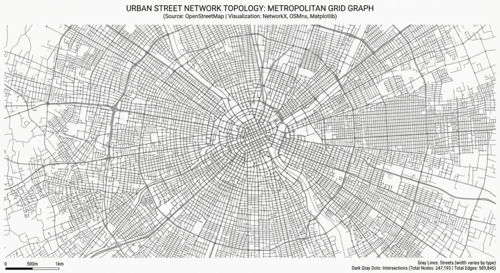
Visual output: The image shows the spatial arrangement of street segments and intersections. Dense street patterns may indicate compact urban development, while sparse patterns may reflect lower-density development or less complete mapping.

The map should be interpreted alongside the network statistics, not as proof of connectivity or accessibility by itself.

6.2 Highlight the calculated route

if route is not None:
    # Draw the selected route on the street network.
    fig, ax = ox.plot.plot_graph_route(
        G,
        route,
        route_color="#e11d48",
        route_linewidth=3,
        node_size=0,
        edge_color="#cbd5e1",
        edge_linewidth=0.6,
        bgcolor="white",
        show=False,
        close=False,
    )

    ax.set_title(
        f"Shortest-Distance Route: {route_length_m / 1000:.2f} km"
    )

    # Save the route visualization.
    fig.savefig(
        OUTPUT_DIR / "shortest_route.png",
        dpi=250,
        bbox_inches="tight",
    )

    plt.close(fig)
    print("Shortest-route map exported.")

The selected route appears as a highlighted line over the street network. Use the map to check for implausible detours, gaps in the network, or endpoints located on unsuitable streets.

6.3 Create an interactive Folium map

For interactive reporting, convert the route edges to a GeoDataFrame and display them in a browser-based map.

if route is not None:
    # Convert the route's edges to spatial features.
    route_gdf = ox.routing.route_to_gdf(
        G,
        route,
        weight="length",
    )

    # Create a map centred between the endpoints.
    route_map = folium.Map(
        location=[
            (origin_lat + destination_lat) / 2,
            (origin_lon + destination_lon) / 2,
        ],
        zoom_start=14,
        tiles="OpenStreetMap",
    )

    # Display the route as GeoJSON.
    folium.GeoJson(
        route_gdf.to_json(),
        name="Shortest route",
        style_function=lambda feature: {
            "color": "#e11d48",
            "weight": 5,
            "opacity": 0.95,
        },
    ).add_to(route_map)

    # Mark the origin and destination.
    folium.Marker(
        [origin_lat, origin_lon],
        tooltip="Origin",
    ).add_to(route_map)

    folium.Marker(
        [destination_lat, destination_lon],
        tooltip="Destination",
    ).add_to(route_map)

    # Add the layer selector.
    folium.LayerControl().add_to(route_map)

    # Save the interactive HTML map.
    html_path = OUTPUT_DIR / "shortest_route_interactive.html"
    route_map.save(str(html_path))

    print("Interactive map exported:", html_path)

Open the generated HTML file in a web browser to zoom, pan, and inspect the route.

This version focuses on the route rather than rendering every street segment. For a large urban network, adding all edges as GeoJSON may produce a very large file and slow down the browser.

Provide appropriate OpenStreetMap attribution when publishing maps or distributing outputs derived from OpenStreetMap data. See the OpenStreetMap Foundation attribution guidelines.

7. Real-world applications

7.1 Walkability studies

Street-network analysis helps planners understand how the urban layout affects pedestrian movement and access to essential services.

A practical walkability study can combine:

• Intersection density and physical streets per node.
• Shortest walking distance to schools, clinics, shops, and parks.
• Pedestrian-network gaps and disconnected paths.
• Street centrality and alternative route availability.
• Sidewalk, crossing, slope, and safety information.

For example, calculate the distance from each residential location to its nearest clinic along the pedestrian network, then compare it with straight-line distance. A large difference can indicate that the street layout creates a detour or that a barrier restricts movement.

Intersection density alone should not be treated as a complete walkability score. A highly connected street network may still have unsafe crossings, missing sidewalks, or poor accessibility for people with limited mobility.

7.2 Urban transit accessibility

Network analysis can measure how easily residents can reach public transport stops on foot.

A typical workflow is:

1. Obtain pedestrian street-network data and transit-stop locations.
2. Snap residential origins and stops to appropriate network nodes.
3. Calculate shortest walking distances or estimated travel times.
4. Count the stops reachable within selected distance or time thresholds.
5. Aggregate results by neighbourhood or administrative district.
6. Map areas with limited access to public transport.

A street graph alone does not represent bus timetables, train schedules, service frequency, or transfers. Combine it with a transit dataset such as General Transit Feed Specification (GTFS) when those factors are part of the research question.

8. Common pitfalls and quality-control checks

Incorrect network type: Select a pedestrian, cycling, or driving graph according to the mode being studied.

Inconsistent coordinate systems: Use geographic coordinates for unprojected node searches and projected coordinates for metric spatial analysis.

Misinterpreted graph degree: Distinguish directed graph connections from counts of physical streets.

Inconsistent density calculations: Use matching study boundaries, area units, and intersection definitions when comparing neighbourhoods.

Unrealistic routing costs: A shortest-distance route is not necessarily the fastest, safest, or most accessible route.

Disconnected networks: Check graph components and the effect of retain_all before interpreting failed routes.

Incomplete source data: Validate critical streets and pathways against authoritative local data where possible.

Poor reproducibility: Save the graph, document the retrieval date, record parameters, and retain the output metrics.

Conclusion

OSMnx and NetworkX provide a practical framework for analysing street-network structure and urban accessibility in Python.

The workflow moves from OpenStreetMap network acquisition to graph projection, connectivity measurements, shortest-path routing, and spatial visualization. The resulting metrics and maps can support urban planning, walkability studies, and public-transport accessibility assessments.

The central lesson is that network results are only meaningful when the graph representation, metric definition, and routing cost match the research question. Graph degree differs from physical street connectivity, intersection density depends on its definition, and shortest distance does not necessarily indicate the most accessible route.

By combining network analysis with population, land-use, transport, and pedestrian-infrastructure data, urban data scientists can build more informative and reproducible models of how cities function.

Further reading

• OSMnx documentation — graph construction, projection, network statistics, routing, and visualization.
• OSMnx examples — applied network-analysis notebooks.
• NetworkX shortest-path documentation — weighted routing and shortest-path methods.
• Folium documentation — interactive mapping and GeoJSON layers.
• OpenStreetMap attribution guidelines — attribution for published maps and derived outputs.