Network Analysis GIS Shortest Path: Routing Algorithms and Service Areas Explained

Network Distance vs. Euclidean Distance

• Euclidean Distance (“As the Crow Flies”): Measures the straight-line distance between two points across a continuous two-dimensional surface using the Pythagorean theorem:
  $$d = \sqrt{(x_2 – x_1)^2 + (y_2 – y_1)^2}$$
• Network Distance: Measures movement constrained to a discrete, interconnected linear network (such as roads, railways, or utility pipelines). Movement can only occur along valid network edges, obeying directionality, connectivity rules, and travel costs.

EUCLIDEAN (Straight Line)           NETWORK (Constrained to Road Grid)
       (A)                                 (A)=======[Edge 1]=======┐
        \                                                           ║ [Edge 2]
         \  <-- Ignored Obstacles                                   ║
          \                                                         ▼
          (B)                                (B)<======[Edge 3]=====╝

1. Building a Network Dataset: Topologies and Impedance

A. Edges (Links)

B. Nodes (Junctions)

C. Turn Features and Rules

D. One-Way Restrictions and Directionality

E. Impedance Attributes

• Distance Impedance: Measured in meters or miles (calculates the shortest physical path).
• Time Impedance: Measured in seconds or minutes (calculates the fastest temporal path). Travel time for an edge is calculated as:
  $$\text{Time} = \frac{\text{Length}}{\text{Speed}}$$
• Financial/Energy Cost: Measured in fuel consumption, toll fees, or slope effort.

[From-Node] ─── Edge 101 (Length: 500m, Speed: 50km/h -> Time: 36s) ─── [To-Node]

e

2. Network Analysis GIS Shortest Path: Dijkstra’s Algorithm

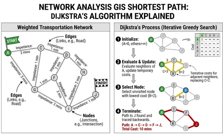
How Dijkstra’s Algorithm Works

   (B) ── [3 mins] ── (D)
  /  \               /
[2 mins] [1 min]  [4 mins]
/      \           /
(S) ── [5 mins] ── (C)

1. Initialization: Assign a tentative distance cost of infinity ($\infty$) to all nodes, and a cost of $0$ to the origin node $S$. Mark all nodes as unvisited. Set $S$ as the current node.
2. Neighbor Evaluation: For the current node, examine all unvisited neighboring nodes. Calculate their tentative cumulative costs through the current node:
   $$\text{Tentative Cost} = \text{Current Node Cost} + \text{Edge Impedance}$$
3. Cost Update: If the calculated tentative cost is less than the neighbor’s currently recorded cost, update the neighbor’s cost to this lower value and record the current node as its predecessor.
4. Node Selection: Once all neighbors of the current node are evaluated, mark the current node as visited. A visited node is never re-evaluated.
5. Iteration: Select the unvisited node with the lowest tentative cost as the new “current node” and repeat steps 2–4.
6. Termination: The algorithm terminates when the destination node is marked as visited or when all reachable nodes have been processed. The final route is reconstructed by tracing backwards through the predecessor nodes.

3. Generating Service Areas and Catchment Zones

Service Areas vs. Standard Proximity Buffers

• Standard Euclidean Buffers: Draw perfect circular zones around a point based on straight-line distance. They completely ignore road layouts, physical barriers (rivers, railways), and directional restrictions.
• Network Service Areas (Isochrones): Measure distance or travel time outwards from a facility along valid network edges up to a specified maximum impedance limit (e.g., 5-minute, 10-minute, or 15-minute cutoffs). The extremities of these edge travel limits are then joined to form realistic catchment polygons.

CIRCULAR EUCLIDEAN BUFFER           NETWORK SERVICE AREA (ISOCHRONE)
       ┌─────────┐                                 ▲
    ┌──│─── 10m ──│──┐                             ║ 10-min drive
    │  │   (C)   │  │                       ◄═════(C)═════►
    └──│─────────│──┘                              ║
       └─────────┘                                 ▼
 (Overestimates real access)             (Accurate street access)

Key Applications of Service Areas

1. Emergency Service Coverage: Mapping areas accessible within 8 minutes from fire stations to evaluate compliance with public safety standards.
2. Retail Catchment Analysis: Determining the population live-work density within a 15-minute walk of a prospective supermarket site.
3. Urban Equity & Planning: Identifying “transit deserts” or areas lacking 10-minute walking access to primary healthcare clinics.

4. Practical Application: Hospital Access & Ambulance Routing

Scenario Brief

An urban healthcare facility needs to assess emergency service coverage across a city. You are given a city road network layer, a location layer for emergency response stations, and a layer of emergency calls.

Task 1: Calculate the fastest route for an ambulance from Station A to Emergency Call #104.

Task 2: Generate 5-minute and 10-minute response catchment zones around all station locations to highlight underserved neighborhoods.

                 [ City Road Network ]
                           │
             ┌─────────────┴─────────────┐
             ▼                           ▼
[ Task 1: Route Solver ]    [ Task 2: Service Area Solver ]
             │                           │
  • Impedance: Travel Time    • Cutoffs: 5 & 10 Minutes
  • Impedance Attribute:      • Output: Overlapping
    Minutes (Length/Speed)      Isochrone Polygons
  • Obstacle: Closed Bridge              │
             │                           ▼
             ▼                [ Underserved Zone Map ]
 [ Optimized Route Layer ]

Analytical Steps for Your GIS Assignment

1. Data Pre-processing & Topological Verification: Inspect the road layer to confirm clean node-edge connections. Ensure fields for Length_m, Speed_kmh, and DriveTime_min are calculated properly.
2. Defining Impedance Attributes: Configure the network solver to use DriveTime_min as the primary cost attribute instead of physical length.
3. Setting Restrictions: Apply one-way attributes (OneWay = 'FT' or 'TF') and add temporary point line barriers (e.g., a closed bridge undergoing maintenance).
4. Executing Route Optimization: Run the shortest path solver to route the ambulance. The solver applies Dijkstra’s algorithm, navigating around the bridge barrier and utilizing high-speed arterial roads to minimize travel time rather than total meters driven.
5. Executing Service Area Analysis: Run the service area solver using 5-minute and 10-minute cutoffs. The resulting isochrone maps reveal neighborhoods situated beyond a 10-minute response envelope, providing empirical evidence for your lab report recommendations.

5. Software Workflow Summary: ArcGIS Pro vs. QGIS

ArcGIS Pro (Network Analyst Extension)

1. Creating the Network Dataset

• Navigate to the Catalog Pane $\rightarrow$ Right-click your Geodatabase Feature Dataset $\rightarrow$ Select New $\rightarrow$ Network Dataset.
• Follow the wizard to set up connectivity rules, elevation fields, turn rules, and cost attributes (Minutes, Meters).
• Click Build Network Dataset in the Geoprocessing pane to index nodes and edges.

2.  Performing a network analysis gis shortest path Calculation in ArcGIS

• Go to the Analysis tab on the top ribbon $\rightarrow$ Click Network Analysis $\rightarrow$ Select Route.
• In the Network Analyst contextual ribbon, click Import Stops to load your origin and destination points.
• Set Travel Mode to Driving Time or Driving Distance.
• Click Run to generate the optimal polyline route and turn-by-turn directions.

3. Generating Service Areas

• Go to Analysis $\rightarrow$ Network Analysis $\rightarrow$ Select Service Area.
• Click Import Facilities to load point locations (e.g., fire stations).
• In the Service Area tab, enter your Cutoffs (e.g., 5 10 15).
• Select Output Type (Polygons) and Geometry Type (Overlapping or Dissolved), then click Run.

Before running any network analysis gis shortest path calculation in ArcGIS Pro, ensure your network dataset topological layers are fully built and indexed.

QGIS (Native & Plugin Workflows)

1. Shortest Path via Native Network Analysis

• Open the Processing Toolbox panel (Ctrl + Alt + T).
• Expand Network Analysis $\rightarrow$ Double-click Shortest Path (Point to Point) or Shortest Path (Layer to Point).
• Select your vector road layer under Vector Layer Representing Network.
• Set Path Type to Calculate to Shortest (Distance) or Fastest (Time).
• Specify start and end points directly on the map canvas and click Run.

2. Advanced Routing & Isochrones via ORStools / QNEAT3

• Install the ORStools plugin (uses OpenRouteService API) or QNEAT3 plugin (QGIS Network Analysis Toolbox 3) via the Plugins Manager.
• For Isochrones (QNEAT3): Go to Processing Toolbox $\rightarrow$ QNEAT3 $\rightarrow$ Isochrones $\rightarrow$ Select Isochrone Area (from Layer).
• Set your input points layer, select the road network layer, define your maximum speed field, set time cost limits (in seconds), and click Run to output vector catchment polygons.

Conclusion: Network Modeling in Real-World Spatial Planning