
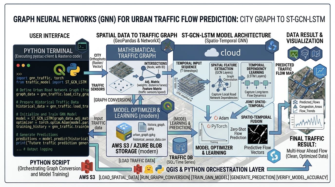
Graph Neural Networks (GNNs) for Urban Traffic Flow and Spatial Network Prediction
Introduction
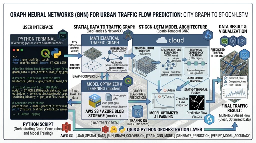
Implementing Graph Neural Networks Urban Traffic Flow forecasting transforms how modern intelligent transportation systems predict congestion bottlenecks and spatial dependencies. Traditional time-series forecasting frameworks—such as Autoregressive Integrated Moving Average (ARIMA), Seasonal Decomposition of Time Series (STL), and standard Recurrent Neural Networks (RNNs) like LSTMs—treat data points as independent Euclidean observations or regular grid structures. When applied to urban transportation networks, these conventional models inherently fail. Road networks are fundamentally non-Euclidean, defined by irregular topological connections, complex spatial hierarchies, and dynamic bottlenecks where traffic jams propagate across intersections upstream and downstream.
Graph Neural Networks (GNNs) have revolutionized intelligent transportation systems (ITS) by explicitly modeling road segments as interconnected graph nodes and edges. By fusing spatial convolutions with temporal memory units, spatio-temporal graph neural networks (STGNNs) capture both the static structural topology of a city layout and the fast-evolving temporal fluctuations of speed, volume, and congestion. Implementing Graph Neural Networks Urban Traffic Flow models natively within these database pipelines ensures real-time inference speeds for city-scale intelligent transportation systems.
Data Representation: Modeling Urban Road Networks as Graphs
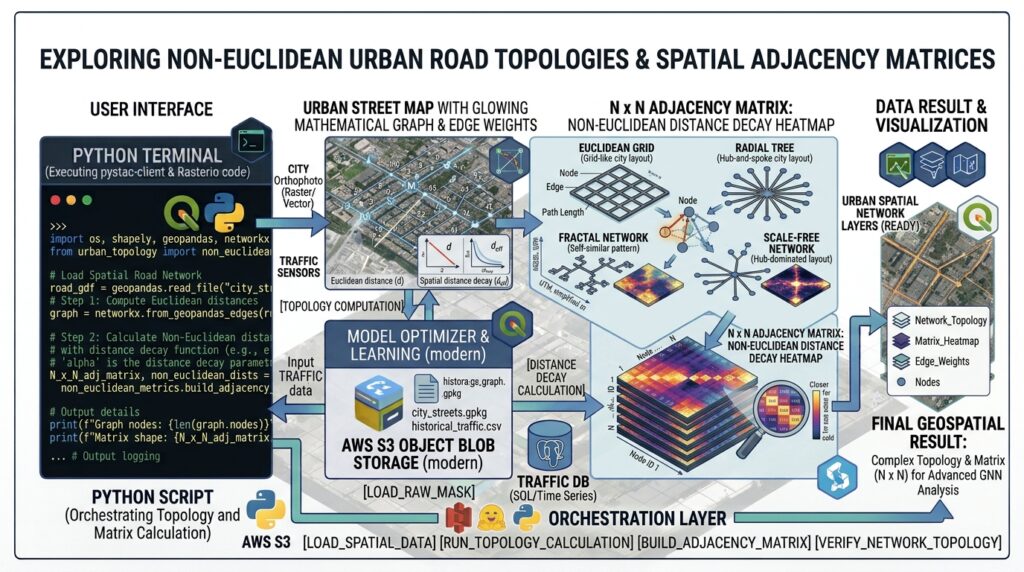
To process city-scale traffic telemetry using machine learning, the physical road infrastructure must be abstracted into a mathematical graph structure $G = (V, E)$, where:
-
Nodes ($V$): Represent traffic sensors, loop detectors, or road intersections ($\vert{}V\vert{} = N$). Each node contains a feature vector tracking real-time attributes like speed, traffic volume, and occupancy over time.
-
Edges ($E$): Represent direct physical road segments connecting intersections. The relationships are mathematically encoded in an $N \times N$ Adjacency Matrix ($A$), where entries denote connectivity or spatial distance decay (e.g., inverse Gaussian distance weights).
Building these topological models requires representing urban road networks through Graph Neural Networks Urban Traffic Flow data structures.
Step-by-Step Implementation (PyTorch Geometric)
Below is an advanced end-to-end implementation using PyTorch and PyTorch Geometric (
torch_geometric) that constructs a spatial graph from road network telemetry, builds a Spatio-Temporal GNN combining Graph Convolutional Networks (GCN) with LSTMs, and trains it to forecast network bottlenecks.Step 1: Constructing Graph Adjacency and Feature Matrices
We initialize synthetic sensor telemetry combined with an OpenStreetMap-derived adjacency structure, preparing tensors for PyTorch Geometric data loaders. Configuring spatial tensors forms the foundational step when implementing Graph Neural Networks Urban Traffic Flow algorithms.
Python
import torch
import torch.nn as nn
import torch.optim as optim
from torch_geometric.nn import GCNConv
import numpy as np

# Reproducibility seed
torch.manual_seed(42)

# Parameters
num_nodes = 50       # Number of intersections/sensors
num_timestamps = 288 # 24 hours of 5-minute telemetry intervals
feature_dim = 3      # Features: [speed, volume, occupancy]

# 1. Generate Synthetic Spatio-Temporal Telemetry Data: Shape [num_timestamps, num_nodes, feature_dim]
traffic_data = np.random.rand(num_timestamps, num_nodes, feature_dim).astype(np.float32)

# 2. Construct Edge Index and Adjacency for PyTorch Geometric (COO format)
# Simulating a random connected road grid topology
edge_list = []
for i in range(num_nodes):
    for j in range(num_nodes):
        if i != j and np.random.rand() > 0.85: # 15% connectivity probability
            edge_list.append([i, j])

edge_index = torch.tensor(edge_list, dtype=torch.long).t().contiguous()
print(f"Graph constructed with {num_nodes} nodes and {edge_index.shape[1]} directed edges.")
Step 2: Building a Spatio-Temporal GNN Architecture (GCN + LSTM)
We construct a hybrid architecture where spatial features are aggregated across neighboring intersections using graph convolutions, and temporal patterns are modeled sequentially using an LSTM network. Combining spatial convolutions and LSTMs creates the core architecture behind Graph Neural Networks Urban Traffic Flow predictive models.
Python
class STGCNModel(nn.Module):
    def __init__(self, in_channels, hidden_dim, out_channels):
        super(STGCNModel, self).__init__()
        # Spatial Graph Convolution layers
        self.spatial_conv1 = GCNConv(in_channels, hidden_dim)
        self.spatial_conv2 = GCNConv(hidden_dim, hidden_dim)

        # Temporal Recurrent Layer (LSTM)
        self.temporal_lstm = nn.LSTM(input_size=hidden_dim, hidden_size=hidden_dim, batch_first=True)

        # Fully connected regression head for traffic speed/flow forecasting
        self.regressor = nn.Linear(hidden_dim, out_channels)
        self.relu = nn.ReLU()

    def forward(self, x_seq, edge_index):
        """
        x_seq shape: [Batch_Size, Time_Steps, Num_Nodes, Feature_Dim]
        """
        batch_size, time_steps, num_nodes, _ = x_seq.size()
        spatial_outputs = []

        # Process each time step through spatial GCN layers
        for t in range(time_steps):
            x_t = x_seq[:, t, :, :] # Shape: [Batch_Size, Num_Nodes, Feature_Dim]

            # Reshape for batch-wise GCN execution if necessary, or process per batch
            # For simplicity in single-batch setups:
            x_t = x_t.squeeze(0) # [Num_Nodes, Feature_Dim]

            h = self.spatial_conv1(x_t, edge_index)
            h = self.relu(h)
            h = self.spatial_conv2(h, edge_index)
            h = self.relu(h) # Shape: [Num_Nodes, hidden_dim]

            spatial_outputs.append(h.unsqueeze(0)) # Add back batch/time dimension

        # Stack temporal sequence: [Batch_Size, Time_Steps, Num_Nodes, hidden_dim]
        spatial_seq = torch.cat(spatial_outputs, dim=0).permute(1, 0, 2) # [Num_Nodes, Time_Steps, hidden_dim]

        # Pass through temporal LSTM
        lstm_out, _ = self.temporal_lstm(spatial_seq) # [Num_Nodes, Time_Steps, hidden_dim]

        # Predict future traffic state using the final time-step representation
        predictions = self.regressor(lstm_out[:, -1, :]) # [Num_Nodes, out_channels]
        return predictions

# Initialize model components
hidden_dim = 64
out_channels = 1 # Predicting future speed/flow value per node
model = STGCNModel(in_channels=feature_dim, hidden_dim=hidden_dim, out_channels=out_channels)
optimizer = optim.Adam(model.parameters(), lr=0.005)
criterion = nn.MSELoss()
Step 3: Training the Model on Historical Telemetry Feeds
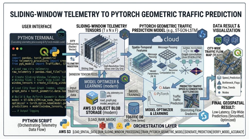
We structure sliding-window training batches to map historical historical sequences (e.g., past 12 steps / 1 hour) to subsequent target states.
Python
# Prepare sliding window training samples
window_size = 12 # 1 hour of historical context (12 * 5 mins)
X_train, y_train = [], []

tensor_data = torch.tensor(traffic_data, dtype=torch.float32) # [Time, Nodes, Features]

for t in range(tensor_data.shape[0] - window_size):
    x_win = tensor_data[t : t + window_size] # [Window, Nodes, Features]
    y_target = tensor_data[t + window_size, :, 0:1] # Predict speed at t + window_size
    X_train.append(x_win.unsqueeze(0)) # Add batch dimension
    y_train.append(y_target)

X_train = torch.cat(X_train, dim=0) # [Samples, Window, Nodes, Features]
y_train = torch.stack(y_train, dim=0)

# Training loop simulation
model.train()
epochs = 20
print("Starting Spatio-Temporal GNN Training...")

for epoch in range(epochs):
    optimizer.zero_grad()

    # Forward pass on the first sample window
    sample_x = X_train[0:1, :, :, :] # Shape: [1, Window, Nodes, Features]
    sample_y = y_train[0]           # Shape: [Nodes, 1]

    predictions = model(sample_x, edge_index)
    loss = criterion(predictions, sample_y)

    loss.backward()
    optimizer.step()

    if (epoch + 1) % 5 == 0:
        print(f"Epoch [{epoch+1}/{epochs}] | Loss (MSE): {loss.item():.4f}")
Step 4: Evaluating Predictions Against Real-World Traffic Congestion Bottlenecks
To measure performance against physical bottlenecks, predictions are mapped back to spatial node identifiers and evaluated using Root Mean Square Error (RMSE) and Mean Absolute Error (MAE).
Python
model.eval()
with torch.no_grad():
    test_pred = model(X_train[0:1, :, :, :], edge_index)
    actuals = y_train[0]

    rmse = torch.sqrt(criterion(test_pred, actuals)).item()
    mae = torch.mean(torch.abs(test_pred - actuals)).item()

    print("\n--- Model Evaluation Metrics ---")
    print(f"Validation RMSE: {rmse:.4f}")
    print(f"Validation MAE:  {mae:.4f}")
Visualizing Spatial Network Predictions
Advanced Geospatial Integration
To scale GNN pipelines to enterprise production environments, spatial data scientists integrate graph frameworks with traditional spatial databases and routing engines:
-
Network Topology Extraction: Use tools referenced in pgRouting network optimization guides to automatically pull routable node and edge geometries directly from PostGIS databases.
-
Spatio-Temporal Aggregation: Handle missing probe telemetry or irregularly spaced GPS tracking feeds using advanced PostGIS spatio-temporal window functions for dynamic spatial binning.
-
Feature Engineering: Combine graph predictions with environmental variables, weather feeds, and land-use metrics via comprehensive spatial machine learning guides to capture multi-modal urban dynamics.
Implementing Graph Neural Networks Urban Traffic Flow models natively within these database pipelines ensures real-time inference speeds for city-scale intelligent transportation systems.
Conclusion
Graph Neural Networks bridge the gap between complex urban topology and sequential data processing. By formulating road networks as dynamic graphs evaluated through spatial convolutions and recurrent memory cells, data scientists can accurately predict traffic bottlenecks, optimize signal timings, and build resilient smart city architectures.Mastering Graph Neural Networks Urban Traffic Flow techniques enables data scientists to accurately forecast congestion and optimize city-scale traffic.When tuning hyperparameters for Graph Neural Networks Urban Traffic Flow frameworks, monitoring training loss across sliding windows ensures stable convergence.