Automating Drought Monitoring with NDVI, NDWI, and NDDI Time Series in GEE

Introduction

Agricultural drought can develop gradually as rainfall decreases, soil moisture declines, and vegetation becomes stressed. Identifying these changes early helps environmental scientists, agricultural planners, and water-resource managers evaluate potential impacts across large regions.

Satellite remote sensing provides a repeatable way to monitor vegetation conditions without relying exclusively on field observations. Google Earth Engine (GEE) makes this process scalable by combining historical satellite imagery, cloud-based processing, temporal analysis, visualization, and raster exports in one platform.

Three useful spectral indicators are the Normalized Difference Vegetation Index (NDVI), the Normalized Difference Water Index (NDWI), and the Normalized Difference Drought Index (NDDI).

NDVI measures vegetation greenness. NDWI, when calculated from near-infrared and shortwave-infrared reflectance, provides information about vegetation moisture. NDDI combines NDVI and this moisture index into a relative indicator of potential drought stress.

These indices provide complementary information, but they are not interchangeable. NDVI and NDWI describe different spectral characteristics, while NDDI combines their signals. None independently confirms that drought is occurring; harvesting, seasonal growth, land-cover change, and other environmental conditions can produce similar patterns.

This tutorial develops a practical Google Earth Engine drought monitoring NDVI NDWI time series workflow using MODIS surface reflectance. The complete script calculates all three indices, compares observations against historical seasonal conditions, generates anomaly charts, creates an exploratory drought-stress classification, and exports a multi-band GeoTIFF.

1. Understand NDVI, NDWI, and NDDI terminology

Before writing the script, distinguish the three indices and the two common meanings of NDWI.

Index	Formula	Primary interpretation
NDVI	((NIR-Red)/(NIR+Red))	Vegetation greenness and vigor
Gao NDWI, often called NDMI	((NIR-SWIR)/(NIR+SWIR))	Vegetation moisture response
McFeeters NDWI	((Green-NIR)/(Green+NIR))	Open-water detection
NDDI	((NDVI-NDWI)/(NDVI+NDWI))	Combined drought-stress indicator

The distinction between the two NDWI formulations is essential. Gao’s vegetation moisture index uses near-infrared and shortwave-infrared reflectance, whereas McFeeters’ NDWI uses green and near-infrared reflectance to help identify open water. The USGS has documented the inconsistent terminology surrounding near-infrared–shortwave-infrared vegetation moisture indices. See the USGS terminology review.

For this tutorial, NDDI is calculated using NDVI and Gao’s NDWI formulation:

[
NDDI=\frac{NDVI-NDWI_{\text{Gao}}}{NDVI+NDWI_{\text{Gao}}}
]

Higher NDDI values can indicate drier vegetation conditions under suitable conditions, but interpretation depends on the index formulation, vegetation type, and local calibration. The denominator must also be sufficiently different from zero to prevent unstable calculations.

The article therefore calculates the following outputs:

• NDVI: indicates vegetation greenness.
• NDWI-Gao (NDMI): indicates vegetation moisture response.
• NDWI-McFeeters: provides an additional open-water indicator.
• NDDI: combines NDVI and the Gao moisture index into a drought-screening indicator.

This approach supports a more complete drought-monitoring workflow than calculating NDVI and NDWI without combining them.

2. Select the satellite dataset and study area

The workflow uses MODIS/061/MOD09A1, the Terra MODIS Surface Reflectance 8-Day Global 500 m product. It provides atmospherically corrected surface reflectance composites at a nominal spatial resolution of 500 metres and has a long historical record suitable for regional monitoring.

The Google Earth Engine Data Catalog documents the available bands and their scale factors.

MODIS band	Spectral region	Application
sur_refl_b01	Red	NDVI
sur_refl_b02	Near-infrared	NDVI and NDWI-Gao
sur_refl_b04	Green	NDWI-McFeeters
sur_refl_b06	Shortwave infrared 1	NDWI-Gao
StateQA	Quality flags	Cloud and observation screening

The reflectance bands use a scale factor of 0.0001. The ratio indices are theoretically independent of a common multiplicative scale factor, but applying the documented scaling makes the reflectance values easier to interpret and use in additional calculations.

MODIS is appropriate for regional drought surveillance because of its frequent observations and extensive archive. Its 500-metre pixels, however, may combine cropland, soil, settlements, and other land-cover types. Sentinel-2 or Landsat may be more suitable where agricultural fields are small or detailed field-level analysis is required.

For a study area, use an agricultural-zone boundary, county polygon, watershed, or collection of farm districts. The example script uses a rectangle over central Kenya. Replace it with your own study geometry before using the outputs for scientific interpretation.

3. Set up Google Earth Engine

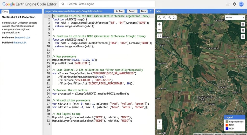
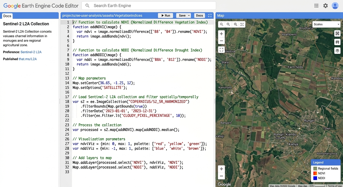
Open the Google Earth Engine Code Editor and create a new JavaScript script.

The example uses a historical baseline from 2001 through 2020 and a monitoring period ending in 2025. The selected target season is January–March 2025.

These dates are illustrative. Change them to match your analysis period, and use a baseline that covers the required observations. To distinguish drought anomalies from normal seasonal variation, compare the target season against the same calendar season in the historical baseline.

4. Complete GEE script: Calculate NDVI, NDWI, and NDDI

The following script calculates all three primary indices and the additional open-water index. It also generates monthly anomalies, standardized anomaly layers, seasonal results, a drought-stress screening map, and a GeoTIFF export.

// ============================================================
// AUTOMATED DROUGHT MONITORING WITH NDVI, NDWI AND NDDI
// Dataset: MODIS/061/MOD09A1
// Platform: Google Earth Engine JavaScript Code Editor
// ============================================================

// 1. CONFIGURATION
// Replace with your own agricultural study boundary.
var region = ee.Geometry.Rectangle([
  36.2, -1.8, 37.4, -0.3
]);

var START_YEAR = 2001;
var END_YEAR = 2025;

var BASELINE_START = 2001;
var BASELINE_END = 2020;

var ANALYSIS_YEAR = 2025;

// End month is exclusive: 1 to 4 means January-March.
var SEASON_START_MONTH = 1;
var SEASON_END_MONTH_EXCLUSIVE = 4;

var SCALE = 500;

// 2. LOAD MODIS SURFACE REFLECTANCE
var raw = ee.ImageCollection('MODIS/061/MOD09A1')
  .filterBounds(region)
  .filterDate(
    ee.Date.fromYMD(START_YEAR, 1, 1),
    ee.Date.fromYMD(END_YEAR + 1, 1, 1)
  );

// 3. QUALITY SCREENING AND SPECTRAL INDICES
function addIndices(image) {
  var qa = image.select('StateQA');

  // StateQA screening:
  // Bits 0-1: cloud state
  // Bit 2: cloud shadow
  // Bits 6-7: aerosol quantity
  // Bits 8-9: cirrus
  // Bit 10: internal cloud flag
  // Bit 12: snow
  // Bit 13: adjacent-to-cloud flag
  var clear = qa.bitwiseAnd(3).eq(0)
    .and(qa.rightShift(2).bitwiseAnd(1).eq(0))
    .and(qa.rightShift(6).bitwiseAnd(3).lt(3))
    .and(qa.rightShift(8).bitwiseAnd(3).eq(0))
    .and(qa.rightShift(10).bitwiseAnd(1).eq(0))
    .and(qa.rightShift(12).bitwiseAnd(1).eq(0))
    .and(qa.rightShift(13).bitwiseAnd(1).eq(0));

  var reflectance = image.select([
    'sur_refl_b01',
    'sur_refl_b02',
    'sur_refl_b04',
    'sur_refl_b06'
  ]).multiply(0.0001).updateMask(clear);

  var red = reflectance.select('sur_refl_b01');
  var nir = reflectance.select('sur_refl_b02');
  var green = reflectance.select('sur_refl_b04');
  var swir = reflectance.select('sur_refl_b06');

  // NDVI = (NIR - RED) / (NIR + RED)
  var ndviDenom = nir.add(red);

  var ndvi = nir.subtract(red)
    .divide(ndviDenom)
    .updateMask(ndviDenom.abs().gt(0.001))
    .rename('NDVI');

  // Gao NDWI / NDMI:
  // (NIR - SWIR1) / (NIR + SWIR1)
  var moistureDenom = nir.add(swir);

  var ndwiGao = nir.subtract(swir)
    .divide(moistureDenom)
    .updateMask(moistureDenom.abs().gt(0.001))
    .rename('NDWI_GAO');

  // McFeeters NDWI for open-water applications:
  // (GREEN - NIR) / (GREEN + NIR)
  var waterDenom = green.add(nir);

  var ndwiMcF = green.subtract(nir)
    .divide(waterDenom)
    .updateMask(waterDenom.abs().gt(0.001))
    .rename('NDWI_MCF');

  // NDDI combines NDVI with the Gao vegetation moisture index.
  var nddiDenom = ndvi.add(ndwiGao);

  var nddi = ndvi.subtract(ndwiGao)
    .divide(nddiDenom)
    .updateMask(nddiDenom.abs().gt(0.05))
    .rename('NDDI');

  return ee.Image.cat([
    ndvi, ndwiGao, ndwiMcF, nddi
  ]).copyProperties(image, ['system:time_start']);
}

var indices = raw.map(addIndices);

print('Input image count:', raw.size());
print('Index collection:', indices.limit(3));

// 4. CREATE MONTHLY INDEX COMPOSITES
var monthly = ee.ImageCollection.fromImages(
  ee.List.sequence(START_YEAR, END_YEAR).map(function(y) {
    y = ee.Number(y);

    return ee.List.sequence(1, 12).map(function(m) {
      m = ee.Number(m);

      var start = ee.Date.fromYMD(y, m, 1);
      var end = start.advance(1, 'month');

      return indices.filterDate(start, end)
        .mean()
        .set({
          year: y,
          month: m,
          'system:time_start': start.millis()
        });
    });
  }).flatten()
);

// 5. CALCULATE MONTH-SPECIFIC HISTORICAL ANOMALIES
function addMonthlyAnomalies(image) {
  var month = ee.Number(image.get('month'));

  var baseline = monthly
    .filter(ee.Filter.gte('year', BASELINE_START))
    .filter(ee.Filter.lte('year', BASELINE_END))
    .filter(ee.Filter.eq('month', month));

  var bands = ['NDVI', 'NDWI_GAO', 'NDDI'];

  var baselineMean = baseline.select(bands).mean();

  var baselineSd = baseline.select(bands)
    .reduce(ee.Reducer.stdDev());

  var ndviAnom = image.select('NDVI')
    .subtract(baselineMean.select('NDVI'))
    .rename('NDVI_anom');

  var ndwiAnom = image.select('NDWI_GAO')
    .subtract(baselineMean.select('NDWI_GAO'))
    .rename('NDWI_anom');

  var nddiAnom = image.select('NDDI')
    .subtract(baselineMean.select('NDDI'))
    .rename('NDDI_anom');

  // Standardized anomalies relative to historical variability.
  var ndviZ = ndviAnom
    .divide(baselineSd.select('NDVI').max(0.02))
    .rename('NDVI_z');

  var ndwiZ = ndwiAnom
    .divide(baselineSd.select('NDWI_GAO').max(0.02))
    .rename('NDWI_z');

  var nddiZ = nddiAnom
    .divide(baselineSd.select('NDDI').max(0.02))
    .rename('NDDI_z');

  return image.addBands([
    ndviAnom, ndwiAnom, nddiAnom,
    ndviZ, ndwiZ, nddiZ
  ]).copyProperties(image, [
    'system:time_start', 'year', 'month'
  ]);
}

var monthlyAnomalies = monthly.map(addMonthlyAnomalies);

// 6. CHART MONTHLY NDVI AND VEGETATION MOISTURE ANOMALIES
var monitoringSeries = monthlyAnomalies
  .filter(ee.Filter.gt('year', BASELINE_END));

var vegetationChart = ui.Chart.image.series({
  imageCollection: monitoringSeries.select([
    'NDVI_anom', 'NDWI_anom'
  ]),
  region: region,
  reducer: ee.Reducer.mean(),
  scale: SCALE,
  xProperty: 'system:time_start'
}).setOptions({
  title: 'Monthly NDVI and vegetation moisture anomalies',
  hAxis: {title: 'Date', format: 'yyyy-MM'},
  vAxis: {title: 'Index anomaly'},
  lineWidth: 2,
  pointSize: 2
});

print(vegetationChart);

// NDDI has a different numerical behavior, so chart it separately.
var nddiChart = ui.Chart.image.series({
  imageCollection: monitoringSeries.select(['NDDI_z']),
  region: region,
  reducer: ee.Reducer.mean(),
  scale: SCALE,
  xProperty: 'system:time_start'
}).setOptions({
  title: 'Standardized NDDI anomaly',
  hAxis: {title: 'Date', format: 'yyyy-MM'},
  vAxis: {title: 'NDDI anomaly (standard deviations)'},
  lineWidth: 2,
  pointSize: 2
});

print(nddiChart);

// 7. CREATE TARGET-SEASON COMPOSITE
var seasonStart = ee.Date.fromYMD(
  ANALYSIS_YEAR, SEASON_START_MONTH, 1
);

var seasonEnd = ee.Date.fromYMD(
  ANALYSIS_YEAR, SEASON_END_MONTH_EXCLUSIVE, 1
);

var currentSeason = indices
  .filterDate(seasonStart, seasonEnd)
  .mean();

var seasonalBaseline = ee.ImageCollection.fromImages(
  ee.List.sequence(BASELINE_START, BASELINE_END)
    .map(function(y) {
      y = ee.Number(y);

      var start = ee.Date.fromYMD(
        y, SEASON_START_MONTH, 1
      );

      var end = ee.Date.fromYMD(
        y, SEASON_END_MONTH_EXCLUSIVE, 1
      );

      return indices.filterDate(start, end)
        .mean()
        .set('year', y);
    })
);

var bands = ['NDVI', 'NDWI_GAO', 'NDDI'];

var seasonalMean = seasonalBaseline.select(bands).mean();

var seasonalSd = seasonalBaseline.select(bands)
  .reduce(ee.Reducer.stdDev());

// Seasonal absolute anomalies.
var ndviAnomaly = currentSeason.select('NDVI')
  .subtract(seasonalMean.select('NDVI'))
  .rename('NDVI_anomaly');

var ndwiAnomaly = currentSeason.select('NDWI_GAO')
  .subtract(seasonalMean.select('NDWI_GAO'))
  .rename('NDWI_anomaly');

var nddiAnomaly = currentSeason.select('NDDI')
  .subtract(seasonalMean.select('NDDI'))
  .rename('NDDI_anomaly');

// Seasonal standardized anomalies.
var ndviZ = ndviAnomaly
  .divide(seasonalSd.select('NDVI').max(0.02))
  .rename('NDVI_z');

var ndwiZ = ndwiAnomaly
  .divide(seasonalSd.select('NDWI_GAO').max(0.02))
  .rename('NDWI_z');

var nddiZ = nddiAnomaly
  .divide(seasonalSd.select('NDDI').max(0.02))
  .rename('NDDI_z');

// 8. CREATE AN EXPLORATORY STRESS CLASSIFICATION
// 0 = no threshold crossed
// 1 = one vegetation index is <= -1 standard deviation
// 2 = NDVI and NDWI-Gao are both <= -1 standard deviation
// 3 = strong positive NDDI anomaly plus negative vegetation
//     and moisture anomalies.
//
// These are screening classes, not an official drought scale.

var valid = currentSeason.select('NDVI').mask()
  .and(currentSeason.select('NDWI_GAO').mask())
  .and(currentSeason.select('NDDI').mask());

var droughtClass = ee.Image.constant(0)
  .updateMask(valid)
  .where(ndviZ.lte(-1).or(ndwiZ.lte(-1)), 1)
  .where(ndviZ.lte(-1).and(ndwiZ.lte(-1)), 2)
  .where(
    nddiZ.gte(1.5)
      .and(ndviZ.lt(0))
      .and(ndwiZ.lt(0)),
    3
  )
  .rename('drought_class')
  .toByte();

// 9. VISUALIZE THE RESULTS
Map.centerObject(region, 8);

Map.addLayer(
  currentSeason.select('NDVI'),
  {
    min: 0,
    max: 0.8,
    palette: [
      '#8c510a', '#d8b365',
      '#a6d96a', '#1a9850'
    ]
  },
  'Seasonal NDVI'
);

Map.addLayer(
  ndwiAnomaly,
  {
    min: -0.2,
    max: 0.2,
    palette: ['#b2182b', '#f7f7f7', '#2166ac']
  },
  'Vegetation moisture anomaly'
);

Map.addLayer(
  nddiAnomaly,
  {
    min: -0.3,
    max: 0.3,
    palette: ['#2166ac', '#f7f7f7', '#b2182b']
  },
  'NDDI anomaly'
);

Map.addLayer(
  droughtClass,
  {
    min: 0,
    max: 3,
    palette: [
      '#d9e2ec', '#fdae61',
      '#f46d43', '#a50026'
    ]
  },
  'Exploratory drought-stress classes'
);

// 10. EXPORT MULTI-BAND GEOTIFF
var exportImage = ee.Image.cat([
  ndviAnomaly,
  ndwiAnomaly,
  nddiAnomaly,
  ndviZ,
  ndwiZ,
  nddiZ,
  droughtClass
]).clip(region);

Export.image.toDrive({
  image: exportImage,
  description: 'Drought_Indices_' + ANALYSIS_YEAR,
  folder: 'GEE_Drought',
  fileNamePrefix: 'drought_indices_' + ANALYSIS_YEAR,
  region: region,
  scale: SCALE,
  maxPixels: 1e13,
  fileFormat: 'GeoTIFF'
});

print('Monitoring year:', ANALYSIS_YEAR);
print('Historical baseline:', BASELINE_START, BASELINE_END);
print('Target season starts:', seasonStart);
print('Target season ends:', seasonEnd);

Important implementation notes

This script is an end-to-end starting point, but the results still require validation.

The quality-screening function uses MODIS StateQA flags to remove several types of contaminated observations. Before operational use, confirm the bit definitions against the MOD09A1 product documentation and assess whether the selected screening criteria are appropriate for your study area.

The NDDI calculation masks pixels where the denominator is close to zero. This avoids extreme values created by unstable division, especially where vegetation is sparse or the index components have opposing values.

For each monthly composite, the script averages the available 8-day index observations. The seasonal baseline is constructed with the same seasonal window for every baseline year, ensuring that the target is compared with a consistent time period.

5. Generate and interpret seasonal anomaly charts

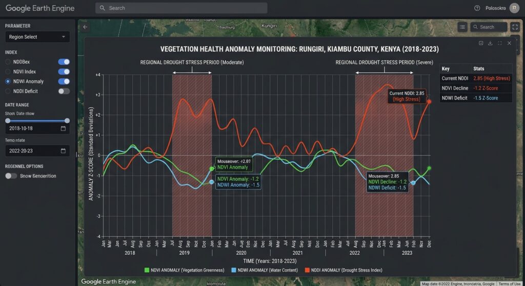
Raw index values naturally vary throughout the year. A healthy crop may have high NDVI during peak growth and lower NDVI after harvesting. An anomaly analysis helps separate these expected seasonal changes from unusual conditions.

For each month, calculate the historical mean:

[
\mu_m=\frac{1}{N}\sum_{y=1}^{N}I_{y,m}
]

where (I_{y,m}) is the index for month (m) in historical year (y).

The absolute anomaly is:

[
A_{y,m}=I_{y,m}-\mu_m
]

A negative NDVI anomaly indicates below-average vegetation greenness for that calendar month. A negative Gao NDWI anomaly suggests lower moisture-index values. A positive NDDI anomaly may indicate a shift toward drier vegetation conditions.

The workflow also calculates standardized anomalies:

[
Z_{y,m}=\frac{I_{y,m}-\mu_m}{\sigma_m}
]

Here, (\sigma_m) is the standard deviation for the matching calendar month in the baseline period.

A standardized anomaly of (-1) means the observation is one historical standard deviation below its baseline mean. A positive NDDI standardized anomaly means NDDI is above its historical average, which can support drought screening when accompanied by negative vegetation and moisture anomalies.

The script generates two charts: one for NDVI and vegetation moisture anomalies, and another for standardized NDDI anomalies. Separating the charts avoids assuming the indices have identical numerical behavior.

Look for sustained anomalies rather than relying on a single observation. Several months of below-average NDVI, declining moisture-index values, and elevated NDDI provide stronger evidence of possible drought stress than an isolated fluctuation. Compare these results with local crop calendars, rainfall deficits, and other independent indicators.

6. Build a drought-stress map and export the results

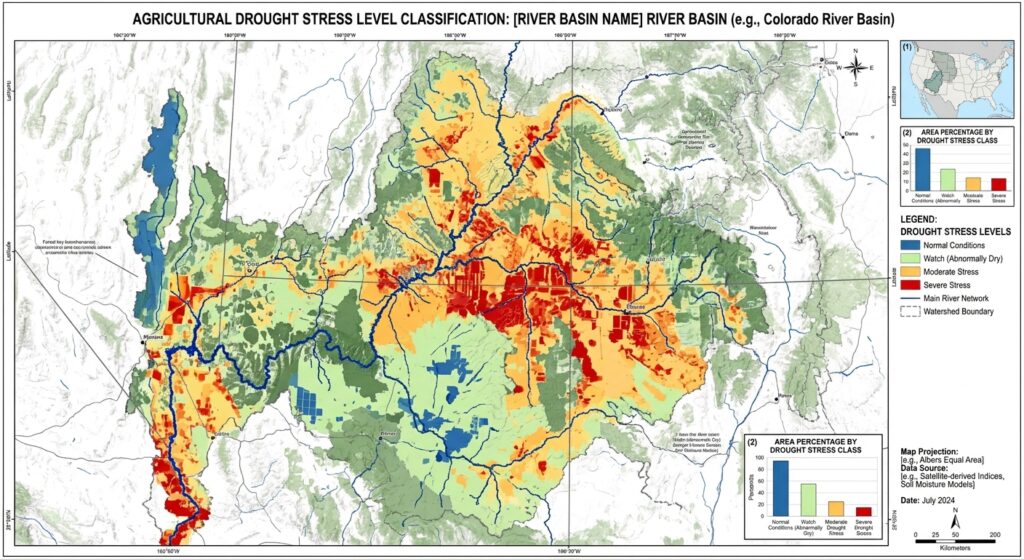
The script produces a screening classification from three sources of evidence: standardized NDVI anomalies, standardized vegetation moisture anomalies, and standardized NDDI anomalies.

Class	Interpretation
0	No selected threshold crossed
1	At least one vegetation or moisture indicator is at or below −1 standard deviation
2	Both NDVI and vegetation moisture anomalies are at or below −1 standard deviation
3	Strong positive NDDI anomaly combined with negative NDVI and moisture anomalies

These categories are configurable analytical flags, not universal drought-severity levels. The threshold values should be adjusted and validated for the crops, climate, and historical variability of the region.

The class 3 condition is designed to identify a stronger combined signal. Because it uses standardized anomalies, it emphasizes deviation from local historical conditions rather than assuming a single absolute NDDI threshold is valid everywhere.

Export the raster

After the script runs, open the Tasks tab and start the Drought_Indices_2025 export. The resulting GeoTIFF includes:

• NDVI_anomaly
• NDWI_anomaly
• NDDI_anomaly
• NDVI_z
• NDWI_z
• NDDI_z
• drought_class

The image export uses the nominal 500-metre resolution of MODIS. See the official Earth Engine image export guide for details.

After downloading the image, open it in QGIS or another GIS and verify the CRS, extent, pixel alignment, NoData regions, and class values. Use diverging color ramps for continuous anomaly layers and a discrete color table for the drought classes.

For recurring monitoring, export one raster per month or reporting season and preserve each run’s baseline years, target dates, input dataset, and threshold configuration. This creates a reproducible archive for agricultural bulletins and regional GIS dashboards.

7. Validate the results before drawing conclusions

Remote-sensing indices alone cannot establish that an agricultural drought is occurring. Validate the workflow with independent information wherever possible.

Observation quality: Inspect cloud contamination, missing pixels, and seasonal data availability. Quality screening reduces contamination but cannot eliminate every observation problem.

Seasonal comparability: Use the same months for the baseline and target. If the region has two growing seasons, calculate separate baselines for the relevant agricultural cycles.

Independent indicators: Compare the results with rainfall anomalies, soil moisture, field surveys, crop condition reports, or established drought indices.

Spatial scale: MODIS pixels may contain several land-cover types. Apply agricultural masks or use Sentinel-2 or Landsat imagery where finer spatial resolution is required.

Threshold calibration: Validate the proposed classes against documented drought events and crop impacts. Avoid presenting the example thresholds as an official or universally transferable severity standard.

Image placeholder

[Image 1: Google Earth Engine time-series chart showing vegetation health anomaly curves during drought periods]

Alt text: “Google Earth Engine chart interface plotting multi-year NDVI, NDWI, and NDDI vegetation health anomaly curves highlighting regional drought stress periods.”

The illustration should display monthly vegetation and moisture anomalies alongside the NDDI anomaly curve, with sustained periods of potential drought stress clearly marked.

SEO best practices and internal linking

Use the primary keyword naturally in the title, introduction, and one relevant heading. Supplement it with related terms such as “automated agricultural drought monitoring,” “satellite vegetation moisture anomalies,” and “multi-year remote sensing analysis.”

Add contextual internal links to related tutorials:

• Time-Series Analysis Using the GEE Python API — automate data retrieval, spatial summaries, and chart generation.
• Multi-Temporal Remote Sensing Change Detection — extend the workflow to land-cover change and long-term environmental monitoring.

Replace the example paths with the actual published URLs on your website.

Conclusion

Google Earth Engine provides a scalable environment for automated drought monitoring using satellite imagery and historical time series. NDVI measures vegetation greenness, Gao’s NDWI formulation provides information about vegetation moisture, and NDDI combines the two into an additional drought-screening indicator.

The workflow in this guide calculates these indices from MODIS surface reflectance, builds seasonal anomalies, charts historical deviations, and exports a multi-band drought-monitoring raster.

The central analytical principle is to interpret the indices together, using consistent historical baselines and independent evidence. Correctly distinguishing the vegetation moisture formulation of NDWI from the open-water formulation—and explicitly calculating NDDI—makes the workflow clearer, more reproducible, and better suited to agricultural drought analysis.

Technical references: MODIS MOD09A1 Data Catalog, Earth Engine image collection charts, Earth Engine image export, USGS vegetation moisture-index terminology, and NDDI application in agricultural drought monitoring.