Table of Contents

Data Classification Methods in GIS: Natural Breaks vs Equal Interval Explained

Introduction to Data Classification Methods in GIS

Data classification methods in GIS determine how numerical values are grouped into classes before they are displayed on a choropleth map. Although the underlying geographic data remains unchanged, changing the class boundaries can produce a very different visual impression.

For example, suppose a map shows unemployment rates for 100 administrative districts. One classification method might place most districts into the lowest two classes, while another might distribute them almost evenly across all five classes. The geographic pattern has not changed—but the visual story presented to the map reader has.

This is why choropleth map classification is not simply a cosmetic choice. The classification method should reflect the distribution of the data and the purpose of the map.

Common classification methods include:

Natural Breaks (Jenks)
Equal Interval
Quantile
Standard Deviation

The key question is:

How are the numerical values distributed, and what do I want the map reader to understand?

1. Natural Breaks (Jenks)

What Is Natural Breaks Classification?

Natural Breaks, also called Jenks Natural Breaks, identifies groups within the data by looking for relatively large differences between adjacent values.

Instead of dividing the numerical range into equal-sized intervals, the method attempts to place observations with similar values in the same class while creating boundaries where there are relatively large gaps in the data.

For example, imagine population-density values:

10, 12, 13, 15, 18, 21, 24, 80, 85, 92, 95

There is a large gap between 24 and 80. Natural Breaks may use this gap as a class boundary.

How Natural Breaks Works

The algorithm searches for class boundaries that:

Keep similar values together.
Minimize variation within each class.
Maximize differences between classes.

Conceptually:

Small differences within classes + large differences between classes = stronger natural groupings.

This makes Natural Breaks particularly useful when the dataset contains obvious clusters or gaps.

Best Uses

Natural Breaks is often appropriate for:

Population density
Property values
Income
Crime rates
Land values
Disease rates
Environmental measurements
Other datasets with clusters or uneven distributions

It is especially useful when the goal is to show patterns inherent in the data.

Advantages

1. Reflects the actual data distribution

Class boundaries are influenced by where the data naturally cluster.

2. Good for skewed datasets

If most observations are concentrated in one range but a smaller number have much higher values, Natural Breaks can separate those groups.

3. Visually emphasizes meaningful differences

Large gaps in the data can become visible class boundaries.

Disadvantages

1. Classes may contain very different numbers of features

One class could contain many districts while another contains only a few.

2. Difficult to compare across multiple maps

Because class boundaries depend on each dataset, two maps may use different breaks even when the same variable is being mapped.

3. Can emphasize extreme values

A few unusually high or low observations can influence the classification.

Example

Suppose five classes are required for a population-density map:

Class	Density
1	0–50
2	51–120
3	121–300
4	301–900
5	901–5,000

These intervals are unequal because they follow gaps and clusters in the data.

2. Equal Interval

What Is Equal Interval Classification?

Equal Interval divides the entire range of values into intervals of equal numerical size.When evaluating data classification methods in gis, Equal Interval works best for datasets with a uniform distribution.

If the minimum value is 0 and the maximum is 100, and you want five classes, the range is divided into five 20-unit intervals:

Class	Range
1	0–20
2	20–40
3	40–60
4	60–80
5	80–100

The number of observations in each class is not considered.

How Equal Interval Works

The basic calculation is:

Class interval = (Maximum − Minimum) ÷ Number of Classes

For example:

Minimum = 10
Maximum = 110
Classes = 5

Therefore:

(110 − 10) ÷ 5 = 20

The resulting classes would cover approximately:

10–30
30–50
50–70
70–90
90–110

Best Uses

Equal Interval works well when:

The data has a relatively uniform distribution.
The numerical magnitude itself is important.
You want the map legend to be easy to understand.
You need straightforward interpretation.
The map communicates thresholds or ranges.

It can be particularly useful for variables such as:

Temperature
Elevation
Rainfall
Index scores
Environmental measurements with relatively regular distributions

Advantages

1. Very easy to understand

The reader can immediately see what each class represents.

2. Preserves numerical magnitude

A difference of 20 units represents the same class width throughout the legend.

3. Useful for comparing maps

If the same class boundaries are deliberately maintained across several maps, comparisons become easier.

Disadvantages

1. Can create empty or sparsely populated classes

If data is strongly skewed, some intervals may contain very few observations.

2. May hide important patterns

Many observations can be concentrated in one or two classes.

3. Sensitive to outliers

An extremely high value can expand the overall range and make the lower classes unnecessarily broad.

Example

Consider income values ranging from KSh 10,000 to KSh 210,000.

With five equal intervals:

Class	Income
1	10,000–50,000
2	50,001–90,000
3	90,001–130,000
4	130,001–170,000
5	170,001–210,000

This is easy to explain, but it may not represent how the population is actually distributed.

3. Quantile Classification

What Is Quantile Classification?

Quantile classification GIS methods divide observations so that each class contains approximately the same number of geographic features.

For example, if a dataset contains 100 counties and you create five classes, Quantile will attempt to place approximately:

100 ÷ 5 = 20 counties per class

The numerical ranges of those classes can therefore be very different.

How Quantile Works

Imagine the sorted values are:

5, 7, 8, 9, 10, 12, 15, 20, 50, 100

With two classes, Quantile would divide the observations into approximately equal groups:

Class 1: lower half
Class 2: upper half

Notice that the numerical difference between observations may not be uniform.

Best Uses

Quantile is useful when you want to show:

Relative ranking
High versus low areas
Percentile groups
Population rankings
Relative socioeconomic conditions
Distribution of features among categories

It is often useful for maps where the question is:

Which areas are among the highest or lowest relative to the others?

Advantages

1. Every class receives approximately the same number of features

This creates a balanced-looking map.

2. Makes relative ranking easy to see

The darkest class represents the highest-ranked observations.

3. Produces good visual contrast

Because classes are populated relatively evenly, most colors are likely to appear on the map.

Disadvantages

1. Can split very similar values

Two areas with almost identical values might end up in different classes.

2. Can group very different values

A class may contain values that are numerically far apart.

3. Can exaggerate small differences

A map can appear to show a strong geographic contrast even when the numerical differences between neighboring classes are small.

Example

Suppose 20 districts are divided into four Quantile classes.

Each class contains approximately five districts:

Class	Approximate Feature Count
Q1	5
Q2	5
Q3	5
Q4	5

However, the numerical ranges could look like:

Class	Value Range
Q1	5–12
Q2	13–18
Q3	19–75
Q4	76–500

This demonstrates an important limitation: equal numbers of features do not mean equal numerical differences.Among the various data classification methods in gis, Quantile classification ensures each class receives an equal number of features.

4. Standard Deviation Classification

What Is Standard Deviation Classification?

Standard Deviation classification organizes observations according to how far they are from the mean.

Instead of simply asking how large a value is, the method asks:

How far above or below the average is this location?

A simplified classification might use boundaries based on:

Below −2 standard deviations
−2 to −1 standard deviations
−1 to 0
0 to +1
+1 to +2
Above +2

The standard deviation measures how widely observations are spread around their mean. Larger standard deviation indicates greater dispersion.

Best Uses

Standard Deviation is particularly useful for:

Statistical analysis
Showing above/below-average areas
Socioeconomic indicators
Demographic variables
Environmental measurements
Identifying unusually high or low values

It is especially useful when the relationship to the mean is more important than the absolute value.

Advantages

1. Highlights deviation from average

The map reader can quickly identify areas substantially above or below the mean.

2. Useful for normally distributed data

Standard deviation is particularly informative when the data approximately follows a bell-shaped distribution.

3. Supports statistical interpretation

The legend directly relates geographic values to the dataset’s statistical characteristics.

Disadvantages

1. More difficult for beginners to interpret

A legend based on standard deviations is less immediately intuitive than simple numerical ranges.

2. Can be misleading with highly skewed data

When the dataset contains strong skewness or extreme outliers, the mean and standard deviation may not represent the distribution well.

3. Requires understanding of statistical variation

The method is most useful when the audience understands what standard deviation represents.

Natural Breaks Jenks vs Equal Interval: Key Differences

These two methods are frequently confused because both can produce five or seven classes, but they answer different questions.

Characteristic	Natural Breaks (Jenks)	Equal Interval
Main principle	Groups similar values	Divides numerical range equally
Uses data distribution?	Yes	No
Class widths	Unequal	Equal
Good for clusters?	Yes	Sometimes
Good for skewed data?	Often	Usually less suitable
Easy to explain?	Moderate	Very easy
Useful for fixed thresholds?	Sometimes	Yes
Sensitive to outliers?	Yes	Yes
Cross-map comparison	More difficult	Easier

Simple way to remember the difference

Natural Breaks asks:

“Where are the natural gaps in my data?”

Equal Interval asks:

“How can I divide the numerical range into equal-sized sections?”

Quick Reference Matrix

The following matrix provides a practical starting point when choosing a classification method.

Method	Best Data Type	Main Strength	Potential Visual Distortion
Natural Breaks (Jenks)	Skewed, clustered	Reveals natural groupings	Can exaggerate clusters and make cross-map comparisons difficult
Equal Interval	Uniform or relatively evenly distributed	Simple numerical interpretation	Can create empty/sparse classes when data is skewed
Quantile	Ranked or moderately skewed data	Equal number of features per class	Can exaggerate small numerical differences
Standard Deviation	Approximately normal	Shows deviation from the mean	Can perform poorly with strongly skewed distributions

Important: There is no universally “correct” classification method. The appropriate method depends on the distribution of the data and the purpose of the map.

Understanding Visual Bias in Choropleth Maps

Classification can influence how a reader interprets geographic patterns.

Consider a dataset where most regions have values between 10 and 30, but a few regions have values above 200.

Different methods can produce very different maps.

Natural Breaks

The large gap between 30 and 200 may become a class boundary.

Potential result: The high-value regions become visually distinct.

Equal Interval

The 0–200 range is divided into equal numerical intervals.

Potential result: Most regions may fall into the lowest class or two classes.

Quantile

The dataset is divided according to feature rankings.

Potential result: The map may show strong color variation even if many numerical values are relatively similar.

Standard Deviation

Values are displayed according to their distance from the mean.

Potential result: Areas substantially above or below average become prominent.

The underlying data is identical in all four cases.

Only the classification changes.

Practical Recommendation: Inspect the Histogram First

Before selecting a classification method, inspect the distribution of your data.

A histogram is one of the most useful tools for making this decision because it shows how frequently values occur across the numerical range.

Step 1: Inspect the Minimum and Maximum

First determine:

Minimum value
Maximum value
Mean
Median
Range
Standard deviation

A large difference between the mean and median can be a warning that the data is skewed.

Step 2: Look for Clusters and Gaps

Ask:

Are there obvious groups?
Are there large gaps between groups?
Are most observations concentrated in one area?
Are there extreme values?

If the histogram contains obvious clusters separated by gaps, Natural Breaks may be worth testing.

Step 3: Look for Skewness

If most values are concentrated toward one end with a long tail extending toward the other end, the dataset is likely skewed.

For example:

10, 11, 12, 13, 15, 17, 19, 25, 80, 250

The values are concentrated at the lower end, with a long upper tail.

In such cases, test Natural Breaks and Quantile rather than automatically choosing Equal Interval.

Using Histograms in ArcGIS Pro

In ArcGIS Pro, you can inspect the distribution of a numeric field before finalizing your symbology.

A typical workflow is:

Open the map containing your layer.
Open the layer’s attribute data.
Identify the numeric field you want to map.
Examine the field’s statistical distribution.
Open the layer’s Symbology pane.
Choose Graduated Colors.
Select the numerical field.
Compare classification methods.
Inspect the class boundaries and resulting map.
Check whether the classes make sense relative to the histogram.

[Insert Screenshot of ArcGIS Pro Graduated Colors Symbology and Histogram]

Do not simply accept the software’s default classification. Examine how changing the classification changes the spatial pattern.

Using Histograms in QGIS

In QGIS, you can inspect the distribution of numerical attributes and then test different graduated symbology classification methods.

A typical workflow is:

Open your GIS project.
Open the layer’s Properties.
Select Symbology.
Choose Graduated.
Select the numerical attribute.
Select an appropriate color ramp.
Choose the number of classes.
Test classification methods such as:
- Equal Interval
- Quantile
- Natural Breaks (Jenks)
- Standard Deviation
Compare the resulting class ranges.
Return to the data distribution and determine whether the chosen classes represent the dataset appropriately.

[Insert Screenshot of QGIS Graduated Symbology Classification Options]

A Practical Decision Workflow

Use this simple decision process when working on a GIS assignment.

Question 1: Does the data contain obvious clusters?

Yes → Test Natural Breaks.

No → Continue evaluating the distribution.

Question 2: Is the numerical range itself important?

Yes → Consider Equal Interval.

For example, if you need classes representing meaningful ranges such as:

0–10
10–20
20–30
30–40

Equal Interval may provide a straightforward legend.

Question 3: Do you want approximately equal numbers of areas in each class?

Yes → Consider Quantile.

This is useful when relative ranking is important.

Question 4: Is comparison with the mean important?

Yes → Consider Standard Deviation.

This is particularly useful for identifying areas that are substantially above or below average.

Example: Choosing a Classification for Population Density

Imagine a GIS student is mapping population density for 50 administrative districts.

After examining the data, they discover:

Most districts have relatively low density.
A few urban districts have extremely high density.
The distribution is strongly right-skewed.
The goal is to identify geographic clusters of high population density.

Equal Interval

May place most districts into the lowest class because the urban districts stretch the maximum value upward.

Quantile

Will distribute districts relatively evenly across the classes, making it easy to identify the highest-ranked districts.

Natural Breaks

May identify a large gap between ordinary districts and highly urbanized districts.

Standard Deviation

Can show which districts are substantially above the overall mean, but the skewed distribution may reduce the usefulness of mean-based interpretation.

For this particular analytical objective, a student should test Natural Breaks and Quantile and compare their results against the histogram, rather than selecting a method simply because it is the default.

Classification Method vs Map Purpose

The same dataset can legitimately be classified differently depending on the question being asked.

Mapping Objective	Method to Consider
Show natural geographic groupings	Natural Breaks
Show simple numerical ranges	Equal Interval
Show relative ranking	Quantile
Show above/below-average values	Standard Deviation
Compare several maps using identical thresholds	Equal Interval or manually defined breaks
Explore an unfamiliar dataset	Test several methods first

These are starting points rather than absolute rules.

Common Mistakes GIS Students Make

1. Always Using the Default Classification

GIS software provides convenient defaults, but a default is not necessarily appropriate for every dataset.

Better approach: Examine the data distribution before selecting the final method.

2. Choosing a Method Because the Map “Looks Better”

A visually attractive map can still communicate a misleading pattern.

Always ask:

Does the classification accurately represent the distribution and purpose of the data?

3. Ignoring Outliers

One extremely large value can dramatically affect Equal Interval classification.

Check the minimum, maximum, histogram, and summary statistics before finalizing your classes.

4. Using Quantile Without Checking Numerical Differences

Quantile guarantees approximately equal numbers of features per class, but the numerical ranges can vary substantially.

Two adjacent classes may have very similar values—or dramatically different ones.

5. Comparing Maps With Different Class Breaks

Suppose Map A uses:

0–20
21–40
41–60

while Map B uses:

0–50
51–100
101–150

Comparing their colors directly can lead to incorrect conclusions.

For temporal or multi-map comparisons, consider using consistent class boundaries.

Best Practice Checklist

Before publishing or submitting a choropleth map, ask:

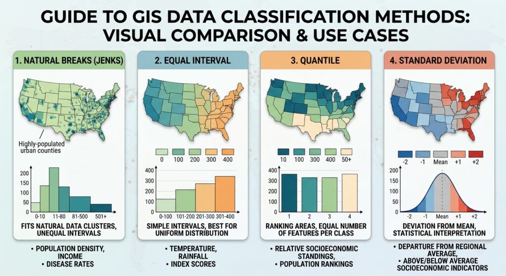
Quick Reference: Which Method Should You Test?

If Your Data Looks Like…	Start By Testing…
Distinct clusters with gaps	Natural Breaks
Relatively uniform distribution	Equal Interval
Strong interest in ranking areas	Quantile
Approximately normally distributed values	Standard Deviation
Strongly skewed distribution	Natural Breaks / Quantile
Several maps requiring direct comparison	Fixed breaks / Equal Interval

Final Takeaway

The choice of data classification methods in GIS can substantially change the visual interpretation of a choropleth map. Natural Breaks, Equal Interval, Quantile, and Standard Deviation each emphasize different characteristics of the same dataset.

The most important distinction is:

Natural Breaks → finds groups within the data.
Equal Interval → divides the numerical range equally.
Quantile → divides observations into similarly sized groups.
Standard Deviation → emphasizes distance from the mean.

For GIS students, the safest workflow is not to ask “Which classification method is the best?” but rather:

“What does my data distribution look like, and which classification method communicates my mapping objective without creating unnecessary visual bias?”

Start with the histogram, test several classification methods, inspect the resulting class boundaries, and document why your final method is appropriate. This turns choropleth classification from a software setting into a defensible cartographic decision.