
Normalized Difference Water Index NDWI vs MNDWI QGIS: A Practical Water Mapping Guide
1. Introduction: Why Map Water Bodies Using Satellite Imagery?
To effectively NDWI vs MNDWI water mapping GIS workflows, it is important to understand. Accurately identifying water bodies from satellite imagery is an important task in hydrology, environmental management, disaster response, and urban planning. Rivers, lakes, reservoirs, wetlands, and floodwater can change in size and location over time. Satellite remote sensing allows researchers to monitor these changes across large areas without conducting field surveys at every location. Learning to perform an **NDWI vs MNDWI water mapping GIS** comparison allows researchers to.
However, water does not always appear clearly separated from other land-cover types in satellite imagery. Urban surfaces, shadows, bare soil, and vegetation can produce spectral responses that complicate water extraction.
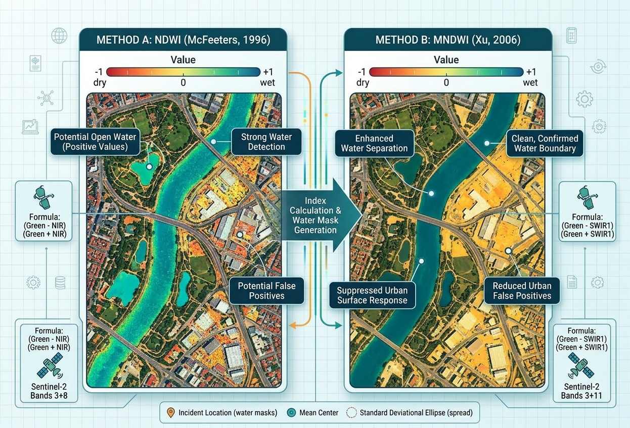
Two widely used spectral indices help address this challenge: the Normalized Difference Water Index (NDWI), introduced by McFeeters in 1996, and the Modified Normalized Difference Water Index (MNDWI), proposed by Xu in 2006.
Both indices use green-band reflectance to enhance open-water features, but they differ in their second band. NDWI uses near-infrared (NIR), whereas MNDWI replaces NIR with shortwave infrared (SWIR).
This seemingly small change can make a substantial difference when mapping water in urban environments.
What is a water index?
A spectral water index combines two satellite bands mathematically to emphasize differences in how water and surrounding surfaces reflect electromagnetic radiation.
Open water generally has relatively strong reflectance in the green band and absorbs much of the incoming energy in the NIR and SWIR regions. Comparing these bands helps distinguish many water pixels from vegetation, soil, and built-up surfaces.
Water indices are useful for:
- Flood management: Identifying inundated areas and monitoring flood extent.
- Drought monitoring: Tracking changes in lakes, reservoirs, and other surface-water features.
- Urban planning: Mapping rivers, ponds, drainage channels, and water bodies in built-up areas.
- Environmental monitoring: Measuring changes in wetlands and inland water features.
- GIS analysis: Producing water masks for area calculations, change detection, and spatial planning.
The important question is not simply which index is better, but which index produces the most reliable results for your study area.
2. Traditional NDWI: McFeeters (1996)
The original NDWI was developed by Stuart K. McFeeters to enhance open-water features and support their delineation from surrounding land cover. It uses green and near-infrared reflectance.
2.1 NDWI formula
The mathematical formula is:
[
\boxed{\mathrm{NDWI}=\frac{Green-NIR}{Green+NIR}}
]
Where:
- Green is reflectance in the visible green band.
- NIR is reflectance in the near-infrared band.
For a typical open-water pixel, green reflectance may be greater than NIR reflectance, producing a positive NDWI value. Vegetation often produces a negative value because its NIR reflectance is relatively strong.
NDWI typically ranges from −1 to +1 when calculated from suitable reflectance data and a non-zero denominator.
A common initial interpretation is that pixels with NDWI greater than zero may represent water. However, zero is only a starting threshold; it is not a universal boundary that perfectly separates water from non-water surfaces.
2.2 Which satellite bands should you use?
The specific bands depend on the satellite sensor.
| Satellite | Green band | NIR band | Typical spatial resolution |
|---|---|---|---|
| Sentinel-2 MSI | B3 | B8 | 10 m |
| Landsat 8/9 OLI | Band 3 | Band 5 | 30 m |
Sentinel-2 B3 and B8 are both 10 m bands. Landsat 8/9 Bands 3 and 5 are both 30 m bands. These matching resolutions simplify pixel-by-pixel calculations. Band specifications are documented by the Copernicus Sentinel-2 documentation and the USGS Landsat 8/9 band guide.
2.3 Advantages of NDWI
NDWI is relatively simple to calculate and can effectively highlight open water in landscapes where water contrasts clearly with surrounding vegetation and soil.
It is particularly useful for rapid water extraction in rural settings, monitoring larger lakes and reservoirs, and generating an initial water mask for further GIS analysis.
Because Sentinel-2’s green and NIR bands are both available at 10 m resolution, the original index can also be useful when spatial detail matters.
2.4 Limitations: Built-up areas can look like water
One of the main limitations of NDWI is confusion between water and certain built-up surfaces.
Concrete, rooftops, roads, and other urban materials may have spectral responses that result in water-like NDWI values. Consequently, NDWI can identify some built-up pixels as potential water, particularly in complex urban environments.
This does not mean NDWI always performs poorly in cities. Its performance depends on surface materials, water conditions, image quality, and the chosen threshold. Nevertheless, the urban-noise problem motivated the development of MNDWI.
Original research: McFeeters (1996), The Use of the Normalized Difference Water Index (NDWI) in the Delineation of Open Water Features.
3. Modified NDWI: Xu (2006)
The Modified Normalized Difference Water Index (MNDWI) was developed by Hanqiu Xu to improve open-water enhancement, particularly in areas where built-up land creates noise in the extracted water layer.
The main modification is straightforward: replace the NIR band in the original NDWI formula with a SWIR band.
3.1 MNDWI formula
[
\boxed{\mathrm{MNDWI}=\frac{Green-SWIR}{Green+SWIR}}
]
Where:
- Green is reflectance in the visible green band.
- SWIR is reflectance in the shortwave infrared region.
In common applications, MNDWI uses SWIR1, rather than SWIR2. The exact band number depends on the satellite.
Water generally absorbs strongly in the SWIR region. Many built-up surfaces and exposed soils show a different green-to-SWIR relationship, enabling MNDWI to suppress some non-water features that complicate the original NDWI.
3.2 Which satellite bands should you use?
| Satellite | Green band | SWIR1 band | Typical spatial resolution |
|---|---|---|---|
| Sentinel-2 MSI | B3 | B11 | 10 m green; 20 m SWIR1 |
| Landsat 8/9 OLI | Band 3 | Band 6 | 30 m for both bands |
For Sentinel-2, B11 has a native resolution of 20 m, while B3 has a native resolution of 10 m. Therefore, a standard MNDWI result should use a common 20 m analysis grid. Resampling B3 to 20 m makes the rasters compatible, but it does not add information to the SWIR image.
For Landsat 8/9, Green Band 3 and SWIR1 Band 6 are both 30 m, making them directly compatible when the grids and extents match. When setting up an **NDWI vs MNDWI water mapping GIS** workflow with Sentinel-2 data, remember B11 is native 20 m.
3.3 Why can MNDWI perform better in cities?
Xu’s modification was designed to enhance open water while suppressing noise from built-up land and other non-water surfaces.
Consider an urban watershed with a river running between roads, buildings, parking areas, and concrete drainage channels. Some of these surfaces may resemble water under the original NDWI. Using SWIR instead of NIR can help separate those surfaces from open water.
MNDWI is therefore often a strong first choice for:
- Urban lakes and reservoirs.
- Rivers running through built-up areas.
- Floodwater mapping in developed landscapes.
- Water-body extraction from scenes containing substantial impervious surfaces.
However, MNDWI does not eliminate every built-up false positive. Building shadows, dark surfaces, turbid water, shallow water, and mixed pixels can still cause classification errors. The best index should be selected through comparison with reference data.
Original research: Xu (2006), Modification of Normalised Difference Water Index (NDWI) to Enhance Open Water Features in Remotely Sensed Imagery.
4. NDWI vs MNDWI: Direct Comparison
The most important difference between the two indices is the second spectral band. That choice affects how strongly each index separates water from surrounding land surfaces. Validating outputs during an **NDWI vs MNDWI water mapping GIS** project requires high-resolution reference data.
| Comparison factor | NDWI — McFeeters | MNDWI — Xu |
|---|---|---|
| Formula | (Green − NIR) / (Green + NIR) | (Green − SWIR1) / (Green + SWIR1) |
| Band combination | Green + NIR | Green + SWIR1 |
| Sentinel-2 bands | B3 + B8 | B3 + B11 |
| Landsat 8/9 bands | B3 + B5 | B3 + B6 |
| Urban-noise suppression | Can confuse some built-up surfaces with water | Often suppresses built-up noise more effectively |
| Rural open-water mapping | Useful where land and water are spectrally distinct | Also useful; performance depends on local conditions |
| Urban flood mapping | Can require additional filtering or careful thresholding | Often a strong starting choice |
| Spatial resolution with Sentinel-2 | 10 m when using B3 and B8 | Usually 20 m because B11 is 20 m |
| Accuracy | Depends on the sensor, site, threshold, and reference data | Depends on the sensor, site, threshold, and reference data |
Which index should you choose?
For a relatively simple rural lake or reservoir, start with NDWI and compare the extracted boundary with an existing water layer.
For a city, industrial zone, or urban floodplain containing extensive impervious surfaces, start with MNDWI because its SWIR band often suppresses built-up noise more effectively.
For a formal research project, calculate both indices and compare their classification results against reference water boundaries, high-resolution imagery, or field observations. Neither index is automatically more accurate in every environment.
5. Step-by-Step QGIS Walkthrough: Extract Water Bodies
This workflow demonstrates how to calculate NDWI and MNDWI using the QGIS Raster Calculator, then create preliminary water masks.
Step 1: Download and prepare satellite imagery
Obtain a cloud-free satellite image covering your area of interest.
Useful sources include:
- Copernicus Data Space Browser for Sentinel-2 imagery.
- USGS EarthExplorer for Landsat imagery.
Where possible, use atmospherically corrected surface reflectance products. Mask clouds and cloud shadows before calculating the indices, as contamination can distort spectral values.
For Sentinel-2, download B3, B8, and B11. For Landsat 8/9, download Bands 3, 5, and 6.
For Landsat Collection 2 Level-2 surface reflectance, apply the documented scale factor and offset before calculating normalized-difference indices:
[
\rho = DN \times 0.0000275 – 0.2
]
where (\rho) is surface reflectance and (DN) is the stored digital number. For Sentinel-2, check the product metadata for the appropriate reflectance scaling. Do not assume every downloaded raster already contains reflectance values on a 0–1 scale.
Step 2: Load raster bands into QGIS
- Open QGIS and create a new project.
- Select Layer → Add Layer → Add Raster Layer.
- Browse to the downloaded band files and load them.
- Rename the layers clearly.
For a Sentinel-2 project, for example, use:
Green_B3NIR_B8SWIR1_B11
Check the raster CRS, extent, and pixel size. NDWI inputs must use a compatible grid. MNDWI inputs must also share a compatible grid, and Sentinel-2 B3 should be aligned to the 20 m B11 grid for the typical MNDWI workflow.
Step 3: Calculate NDWI using Raster Calculator
Open Raster → Raster Calculator.
In the expression box, enter the following formula, replacing the example names with the names shown in your QGIS raster-band list:
("Green_B3@1" - "NIR_B8@1") /
("Green_B3@1" + "NIR_B8@1")
Set the output path to NDWI.tif, choose an appropriate output extent and resolution, and run the calculation.
The raster calculator processes the formula pixel by pixel. QGIS writes the output to a new raster layer. The QGIS Raster Calculator documentation explains how raster expressions and output settings work.
Quality check: Inspect the raster for unexpected gaps, extreme values, or artefacts. Pixels where the denominator is zero require careful handling. Ensure the input layers use appropriately scaled reflectance values and that cloud masks have been applied.
Step 4: Calculate MNDWI using Raster Calculator
Open Raster → Raster Calculator again.
For Sentinel-2, use B3 and B11:
("Green_B3@1" - "SWIR1_B11@1") /
("Green_B3@1" + "SWIR1_B11@1")
For Landsat 8/9, use Bands 3 and 6:
("Band3_Green@1" - "Band6_SWIR1@1") /
("Band3_Green@1" + "Band6_SWIR1@1")
Save the output as MNDWI.tif and run the calculation.
If you use Sentinel-2, the native SWIR1 band determines the effective spatial detail of a standard 20 m MNDWI workflow. To compare NDWI and MNDWI fairly, align their grids and assess them at a common resolution.
Step 5: Style and compare the index rasters
For each index, right-click the output layer and select Properties → Symbology.
Choose Singleband pseudocolor or an appropriate single-band renderer and use a colour ramp that makes positive and negative values easy to distinguish.
A diverging colour ramp centred near zero is a useful starting point. The display colours are for visual interpretation; they do not change the index values.
Compare both maps against a true-colour image or a suitable false-colour composite. Look for whether the indices highlight known rivers and lakes, and whether roads, buildings, shadows, or bare soil appear as false water features.
Step 6: Extract a preliminary water mask
A simple starting rule is to classify pixels with index values greater than zero as potential water.
For NDWI, open Raster → Raster Calculator and enter:
"NDWI@1" > 0Save this as NDWI_WaterMask.tif.
For MNDWI, use:
"MNDWI@1" > 0Save this as MNDWI_WaterMask.tif.
The resulting raster typically assigns 1 to pixels satisfying the threshold and 0 to pixels that do not. Confirm how NoData is handled in your calculation so invalid pixels are not inadvertently included in the non-water class.
Important: A zero threshold is a preliminary rule, not a guaranteed water boundary. Adjust the threshold using image interpretation, local conditions, and reference data. For scenes with complex land cover, test several thresholds rather than assuming a single value will work everywhere.
Step 7: Validate the extracted water bodies
Overlay the candidate water mask with a reference water-body layer or other reliable information.
Check whether the mapped boundaries match visible rivers, reservoirs, and lakes. Pay particular attention to dark rooftops, building shadows, wet soil, shallow water, and mixed pixels along shorelines.
Where appropriate, use a reference dataset to calculate classification accuracy. Count correctly and incorrectly classified water and non-water pixels, and report relevant metrics such as precision, recall, and overall accuracy. If you plan to compare the two indices quantitatively, use the same reference samples and a consistent spatial grid for both.
After validation, the water mask can support further GIS work such as estimating lake area, mapping potential flood extent, or comparing surface-water changes between dates.
6. Common Limitations to Remember
Clouds and cloud shadows: Optical indices depend on suitable observations. Cloud masking reduces contamination, but shadows and haze can still affect water extraction.
Turbid or shallow water: Suspended sediment, aquatic vegetation, and bottom reflectance can alter the spectral response and reduce separation from surrounding land.
Built-up surfaces: MNDWI often reduces urban noise more effectively than NDWI, but some impervious surfaces and shadows may still be misclassified.
Mixed pixels: A pixel at a shoreline may contain both water and land, making its index value ambiguous. Coarser imagery can be especially challenging for narrow rivers and small ponds.
Temporal changes: Water boundaries can change with season, rainfall, river flow, and reservoir operation. A classification may represent conditions on the image date rather than a permanent water boundary.
7. Conclusion
NDWI and MNDWI are valuable tools for extracting water bodies from satellite imagery in QGIS. Both use the green band, but the second band determines how they respond to water and surrounding land cover. A well-executed **NDWI vs MNDWI water mapping GIS** analysis provides critical insights for hydrological models.
The original NDWI combines Green and NIR reflectance, making it useful for many open-water mapping tasks. MNDWI combines Green and SWIR1 reflectance and often performs better in urban settings by suppressing some built-up land noise.
To produce a reliable water map, use suitable surface reflectance imagery, apply cloud masks, align raster grids, calculate the index with the correct band combination, and validate the resulting water mask. Treat thresholds as study-specific choices rather than universal rules.
For hydrology and environmental GIS projects, calculating both indices and comparing their performance against reference data is often the most informative approach.