
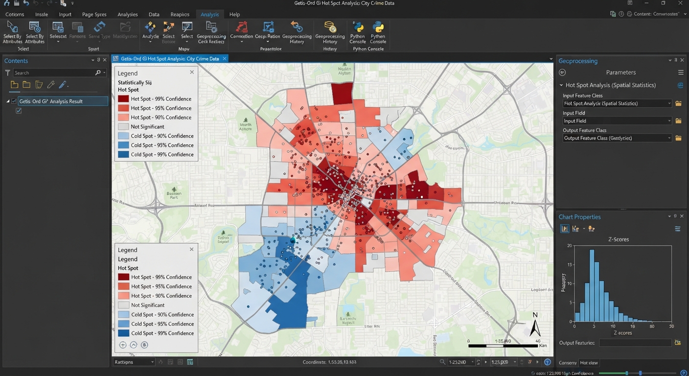
Getis-Ord Gi Hot Spot Analysis GIS Guide: 5 Steps
When examining spatial distributions of phenomena such as crime events, disease outbreaks, traffic accidents, or environmental contamination, visual inspection of point locations can easily be deceiving. A map showing dense clusters of points might simply reflect underlying population density rather than a true statistical anomaly. Performing a Getis-Ord Gi hot spot analysis GIS workflow allows students and spatial analysts to objectively distinguish random geographical occurrences from statistically significant spatial clusters of high values (hot spots) and low values (cold spots). When completing a geography term project, mastering a getis-ord gi hot spot analysis gis workflow is essential for identifying spatial anomalies.
Understanding spatial statistics is a key milestone in upper-level geography, urban planning, public health, and environmental science coursework. This comprehensive step-by-step tutorial covers the mathematical logic behind the $G_i^*$ statistic, guides you through setting spatial weight matrices, demonstrates tool execution in both ArcGIS Pro and QGIS, and highlights best practices for cartographic visualization.
1. Fundamentals of Getis-Ord $G_i^*$ Hot Spot Analysis GIS
The Getis-Ord $G_i^*$ statistic (pronounced G-i-star) evaluates the local value of a feature relative to the values of its neighboring features within a designated distance threshold or neighborhood rule. The mathematical framework behind a getis-ord gi hot spot analysis gis ensures that isolated high-value cells are distinguished from true clusters. When exploring spatial patterns, running a getis-ord gi hot spot analysis gis helps validate visual assumptions statistically.
+-------------------------------------------------------------------------+
|                         INPUT SPATIAL DATASET                           |
|       Point or Polygon Features with Numeric Attribute Values           |
+------------------------------------+------------------------------------+
                                     |
                                     v
                  +-------------------------------------+
                  |   SPATIAL WEIGHTS MATRIX (W_ij)     |
                  | Defines Neighborhood Relationships  |
                  +------------------+------------------+
                                     |
                                     v
                  +-------------------------------------+
                  |       GETIS-ORD G_i* STATISTIC      |
                  |  Compares Local Neighborhood Sum    |
                  |  Against Total Study Area Mean      |
                  +------------------+------------------+
                                     |
            +------------------------+------------------------+
            |                                                 |
            v                                                 v
  High Positive Z-Score                            Low Negative Z-Score
  (Small p-value)                                  (Small p-value)
  [ HOT SPOT CLUSTER ]                             [ COLD SPOT CLUSTER ]
The Logic Behind the Math
A single feature with a high value is not necessarily a statistically significant hot spot. To qualify as a statistically significant hot spot, a feature with a high value must be surrounded by other neighboring features that also exhibit high values.
Mathematically, the $G_i^*$ statistic calculates a $Z$-score and $p$-value for every feature in your dataset:
$$\text{Local Sum} = \sum_{j=1}^{n} w_{i,j} x_j$$
The local sum of a feature and its neighbors is compared proportionally to the global sum of all features across the entire dataset. When the local sum deviates substantially from the expected global sum, a high absolute $Z$-score is produced.
$Z$-Scores, $p$-Values, and Confidence Level Bins
GIS software outputs two main statistical metrics for every feature:
-
$Z$-Score (Standard Deviation): Indicates how far local values deviate from the global mean.
-
$p$-Value (Probability): Measures the likelihood that the observed spatial pattern was created by a random spatial process.
These metrics are categorized into standard confidence level bins:
| Z-Score Range | p-Value Threshold | Statistical Classification | Confidence Level | Map Renderer Color |
| $> +2.58$ | $p < 0.01$ | Hot Spot | 99% Confidence | Dark Red |
| $+1.96 \text{ to } +2.58$ | $p < 0.05$ | Hot Spot | 95% Confidence | Medium Red |
| $+1.65 \text{ to } +1.96$ | $p < 0.10$ | Hot Spot | 90% Confidence | Light Red |
| $-1.65 \text{ to } +1.65$ | $p > 0.10$ | Not Significant | No Cluster | Light Grey / Yellow |
| $-1.96 \text{ to } -1.65$ | $p < 0.10$ | Cold Spot | 90% Confidence | Light Blue |
| $-2.58 \text{ to } -1.96$ | $p < 0.05$ | Cold Spot | 95% Confidence | Medium Blue |
| $< -2.58$ | $p < 0.01$ | Cold Spot | 99% Confidence | Dark Blue |
2. Setting Up Spatial Parameters: Distance Bands & Spatial Weights
Before running the tool, setting appropriate spatial parameter controls is essential to avoid artificial spatial bias. Before calculating neighbors, defining the scale of a getis-ord gi hot spot analysis gis prevents spatial distortion.
Conceptualization of Spatial Relationships
This setting defines how spatial interactions decay or operate across space:
-
Fixed Distance Band (Recommended Default): Every feature is evaluated within a specified fixed search radius ($d$). Features within the distance band are weighted equally ($w_{ij} = 1$). This is ideal for continuous processes or point event analyses.
-
Contiguity Edges Corners (Rook / Queen): Neighbor relationships are determined by shared polygon boundaries. Useful for administrative regions like census tracts or counties.
-
Inverse Distance: Weight decreases continuously as distance between features increases. Best suited for continuous phenomena like temperature or air quality.
Finding the Optimal Distance Threshold
Selecting an arbitrary distance threshold can invalidate statistical results. To calculate an optimal threshold:
-
Run the Incremental Spatial Autocorrelation tool in your GIS suite.
-
Identify the distance value corresponding to the peak Global Moran’s I $Z$-score. This peak represents the spatial scale at which spatial clustering is most pronounced.
3. Step-by-Step Guide: Executing Getis-Ord Gi Hot Spot Analysis GIS in ArcGIS Pro
ArcGIS Pro features native geoprocessing tools under the Spatial Statistics toolbox designed for hot spot detection. Students using ArcGIS Pro will find that running a getis-ord gi hot spot analysis gis automates standard deviation calculations seamlessly. For students submitting lab work, a properly executed getis-ord gi hot spot analysis gis demonstrates strong technical competence.
Step 1: Open the Hot Spot Analysis Tool
-
Launch ArcGIS Pro and load your point or polygon feature dataset.
-
Open the Geoprocessing Pane (Analysis > Tools).
-
Search for and open Hot Spot Analysis (Getis-Ord Gi*) (Spatial Statistics Tools > Mapping Clusters).
Step 2: Configure Tool Parameters
-
Input Feature Class: Select your input spatial layer (e.g.,
Crime_IncidentsorCounty_Health_Data). -
Input Field: Select the numeric attribute field containing the intensity values to evaluate (e.g.,
Incident_CountorInfection_Rate). -
Output Feature Class: Choose your geodatabase destination layer.
-
Conceptualization of Spatial Relationships: Select FIXED_DISTANCE_BAND or CONTIGUITY_EDGES_CORNERS.
-
Distance Band or Threshold Distance: Enter your calculated optimal search distance (or leave blank to allow ArcGIS Pro to auto-calculate a default threshold).
-
Apply FDR Correction: Check the box for False Discovery Rate (FDR) Correction if your dataset contains thousands of features to adjust for multiple testing dependencies.
Step 3: Run and Review Outputs
-
Click Run.
-
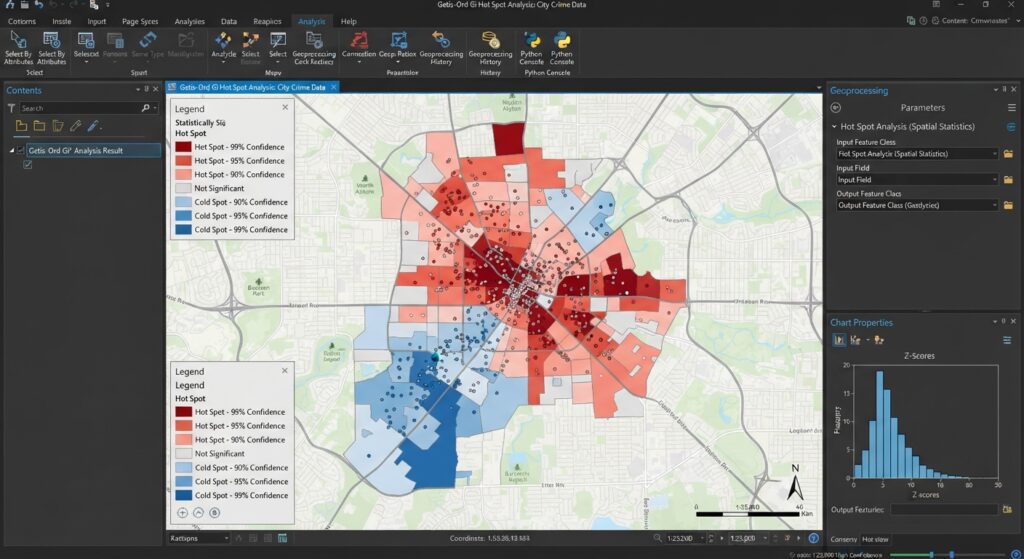
ArcGIS Pro automatically symbolizes the output layer into 7 confidence level categories ranging from -3 (99% Cold Spot) to +3 (99% Hot Spot).
4. Step-by-Step Guide: Executing Getis-Ord Gi Hot Spot Analysis GIS in QGIS
QGIS users can compute Getis-Ord $G_i^*$ statistics using the Hotspot Analysis Plugin or script-based execution via PySAL / PyQGIS. Python scripts in QGIS allow advanced researchers to automate a getis-ord gi hot spot analysis gis efficiently across massive datasets. Automating workflow scripts makes repeating a getis-ord gi hot spot analysis gis across multiple temporal layers efficient.
Method 1: Using the QGIS Hotspot Analysis Plugin
-
Go to Plugins > Manage and Install Plugins.
-
Search for Hotspot Analysis (or spatial statistics plugin) and click Install.
-
Open the plugin from the vector menu (Vector > Hotspot Analysis).
-
Set Input Vector Layer and select your Analysis Field.
-
Choose your neighborhood weighting strategy (Fixed Distance or KNN Nearest Neighbors).
-
Click OK to generate the output spatial vector layer.
Method 2: Python Scripting via PySAL in QGIS
For full control over weights matrix calculation, run PySAL’s
esda module in the QGIS Python Console:Python
import geopandas as gpd
from pysal.explore import esda
from pysal.lib import weights

# Load layer from active QGIS canvas
layer = qgis.utils.iface.activeLayer()
gdf = gpd.read_file(layer.source())

# Generate Spatial Weights Matrix (Fixed Distance Band)
w = weights.DistanceBand.from_dataframe(gdf, threshold=1000, binary=True)

# Calculate Getis-Ord Gi* Statistic
gi = esda.G_Local(gdf['Value_Field'], w, star=True)

# Append Z-scores and p-values to attribute table
gdf['Gi_ZScore'] = gi.Zs
gdf['Gi_PValue'] = gi.p_sim
gdf.to_file(layer.source(), driver="ESRI Shapefile")
Pro Tip: Avoiding Common Spatial Parameter Pitfalls
Effectively communicating statistical results requires clear map design. Follow standard cartographic guidelines when presenting your output:
-
Color Palette: Use a cold-to-hot diverging color scheme (e.g., Dark Blue $\rightarrow$ Light Blue $\rightarrow$ Light Grey $\rightarrow$ Light Red $\rightarrow$ Dark Red).
-
Class Bins: Group attributes into 7 standard confidence bins using the
Gi_Binoutput field:-
+3: Hot Spot – 99% Confidence
-
+2: Hot Spot – 95% Confidence
-
+1: Hot Spot – 90% Confidence
-
0: Not Statistically Significant
-
-1: Cold Spot – 90% Confidence
-
-2: Cold Spot – 95% Confidence
-
-3: Cold Spot – 99% Confidence
-
-
Data Classification Scheme: Do not use Natural Breaks (Jenks) or Equal Interval for $Z$-scores! Apply manual classification based on explicit critical $Z$-score cutoff values ($\pm 1.65, \pm 1.96, \pm 2.58$). For a review of statistical classification techniques, refer to our tutorial on
[Internal Link Context: Suggest linking to related article on Data Classification Methods in GIS]. -
For technical documentation on cluster tool algorithms, check the official Esri Spatial Statistics Documentation.
Proper color rendering on a map created through a getis-ord gi hot spot analysis gis helps communicate statistical findings clearly to evaluators.
6. Frequently Asked Questions (FAQ)
What is the difference between Anselin Local Moran’s I and Getis-Ord Gi*?
Anselin Local Moran’s I identifies spatial clusters (High-High, Low-Low) and spatial outliers (High-Low, Low-High). Getis-Ord $G_i^*$ focuses specifically on identifying statistically significant hot spots (High-High) and cold spots (Low-Low) without isolating spatial outliers.
What does a high positive z-score indicate in hot spot analysis?
A high positive $Z$-score (accompanied by a small $p$-value) indicates a statistically significant spatial cluster of high values (a hot spot). The higher the $Z$-score, the tighter the spatial clustering of high values.
How do I determine the optimal distance threshold for my dataset?
Run the Incremental Spatial Autocorrelation tool in ArcGIS Pro (or plot a variogram/spatial distance decay function) to identify the distance distance where peak spatial autocorrelation ($Z$-score) occurs. Use this distance as your search radius.
7. Conclusion & Summary
Mastering Getis-Ord Gi hot spot analysis GIS techniques bridges the gap between raw spatial data visualization and rigorous statistical inference. By structuring spatial weight matrices, establishing statistically sound distance thresholds, and formatting cartographic outputs, you can deliver professional spatial reports for any university lab assignment. If you ever need professional help with your GIS assignment, mastering hot spot analysis is a great place to start. By following these structural guidelines, your final lab report featuring a getis-ord gi hot spot analysis gis will stand out for its rigorous methodology. Ultimately, mastering a getis-ord gi hot spot analysis gis is an invaluable skill for any spatial data analyst.
Key Takeaways:
-
Always check for projected coordinate systems before calculating distance thresholds.
-
Use Incremental Spatial Autocorrelation to select a distance band based on statistical scale.
-
Symbolize results using standard confidence bins ($\pm 99\%, \pm 95\%, \pm 90\%$).