
Network Analysis in GIS Shortest Path: 2 Powerful Routing Tutorials for Students
Finding the shortest route between two locations sounds simple: identify the two points and calculate the distance between them. However, real transportation networks are more complicated. Network analysis in GIS shortest path workflows consider how roads actually connect and how vehicles move through them, including travel impedance, one-way streets, turn restrictions, and speed limits.
This distinction matters in urban planning, logistics, emergency management, and transportation studies. A straight-line measurement or simple line layer cannot reliably answer questions such as “What is the fastest route?” or “Which neighborhoods are within a 10-minute drive?”
This guide demonstrates two practical network-analysis workflows:
- Finding the shortest or fastest route.
- Creating a 10-minute drive-time service area.
1. Network Analysis in GIS Shortest Path: Key Concepts
Applying network analysis in gis shortest path algorithms allows analysts to model realistic road restrictions rather than simple straight-line distances.
A road shapefile is fundamentally a collection of lines.
A network dataset, however, represents those lines as a connected transportation system with rules and costs. When setting up network analysis in gis shortest path tasks, understanding connectivity rules is crucial for accurate routing.
For example:
| Feature | Standard Road Layer | Network Dataset |
|---|---|---|
| Road geometry | ✓ | ✓ |
| Connectivity | Limited/implicit | Explicit |
| Travel time | Optional attribute | Can be an impedance |
| Speed limits | Optional | Can determine travel time |
| One-way restrictions | Not automatically enforced | Can be modeled |
| Turn restrictions | Usually absent | Can be modeled |
| Shortest path | Basic geometry only | Network-based routing |
| Service areas | No | Yes |
| Closest facility | No | Yes |
A 5 km road may not be the fastest route if another 7 km road has a much higher speed limit.
Similarly, a road that appears connected on a map may not actually be routable if its endpoints do not form a valid network connection.
2. Understanding Network Impedance
Selecting the correct impedance is the most crucial setting in any network analysis in gis shortest path workflow. Incorporating real-world travel delays into your network analysis in gis shortest path model ensures accurate route calculations.
An impedance is the cost that the routing algorithm attempts to minimize.
Common impedance values include:
- Distance
- Travel time
- Fuel cost
- Toll cost
- Generalized transportation cost
For example:
Shortest route
Impedance = DistanceThe solver attempts to minimize total distance.
Fastest route
Impedance = Travel TimeThe solver attempts to minimize estimated travel time.
This means:
Shortest does not necessarily mean fastest.
3. Tutorial 1: Calculate the Shortest or Fastest Path
Using the Network Analyst extension allows you to configure network analysis in gis shortest path solvers based on live road conditions.
Suppose an urban-planning assignment asks:
Find the fastest driving route between a residential area and a hospital.
Your basic workflow is:
Road Network
     ↓
Network Dataset
     ↓
Route Analysis
     ↓
Start + Destination
     ↓
Impedance
     ↓
Solve
     ↓
Optimal Route
Step 1: Prepare the Network Dataset
Before calculating a route, you need a usable transportation network.
In ArcGIS Pro, a network dataset can be constructed from appropriate transportation feature classes.
Typical source data might contain:
Road_ID
Road_Name
Road_Type
Length
Speed_Limit
One_Way
The exact fields depend on the data source and network design.
Step 2: Check Road Connectivity
Before routing, inspect your road network.
Road segments should connect properly at intersections.
For example:
Correct:

──────────────
       │
       │
       │
──────────────


Incorrect:

──────────────

       │
       │
       │
In the second example, the vertical road may visually appear close to the horizontal road but not actually connect to it.
This can create disconnected network edges.
Step 3: Create a Route Analysis Layer
Setting up proper travel modes is essential when configuring network analysis in gis shortest path solvers for transportation studies.
In ArcGIS Pro, create a route analysis layer using the Network Analyst tools.
The route solver will use the network dataset to calculate a path between specified locations.
[Insert Screenshot of Route Analysis Layer / Route Solver Parameters]
Configure the route using an appropriate travel mode and impedance.
For example:
Travel Mode:
Driving

Impedance:
TravelTime
Or:
Travel Mode:
Driving

Impedance:
Length
Step 4: Add the Starting Location
Add the origin point.
For example:
Origin:
Residential Area
This might be:
- A house
- Warehouse
- School
- Fire station
- Hospital
- Distribution center
The point needs to be located close enough to the network for the solver to associate it with a routable road.
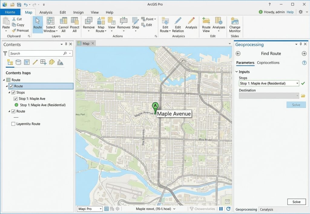
Step 5: Add the Destination
Once your origin and destination points are linked to the network, running a network analysis in gis shortest path calculation becomes straightforward.
Add the destination point.
For example:
Destination:
Hospital
The route solver now has:
Origin
   ↓
Road Network
   ↓
Destination
Step 6: Choose Shortest vs. Fastest
When configuring network analysis in gis shortest path solvers, choosing travel time over physical distance changes the resulting route. This is one of the most important decisions in the analysis.
Shortest path
Choose a distance-based impedance when your research question is:
“What route covers the least distance?”
For example:
Impedance = LengthThe solver minimizes total network distance.
Fastest path
Choose a time-based impedance when your question is:
“What route can be traveled in the least time?”
For example:
Impedance = TravelTimeA longer highway may therefore be selected instead of a shorter residential road.
Example
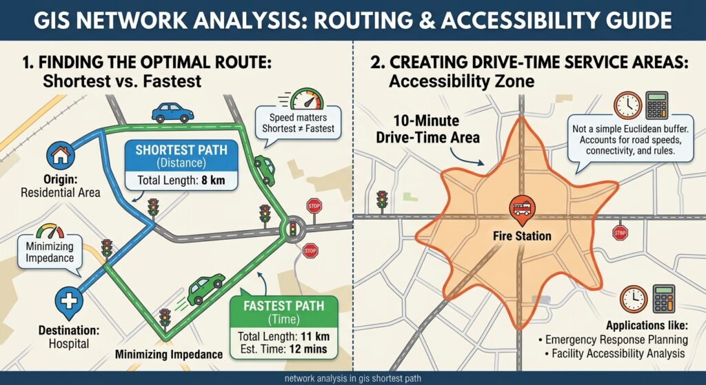
| Route | Distance | Average speed | Approx. time |
|---|---|---|---|
| Route A | 8 km | 30 km/h | 16 min |
| Route B | 11 km | 60 km/h | 11 min |
The shortest route is A.
The fastest route is B.
This is why specifying the correct impedance is essential.
Step 7: Solve the Route
Once the origin, destination, and impedance have been configured, run the route solver.

The resulting route should follow the actual network rather than a straight line.
Conceptually:
Origin ●
       \
        \
         ────────
                 \
                  \
                   ● Destination
The route may contain multiple turns and road segments.
Step 8: Inspect the Route Results
Open the route’s attribute table.
Depending on the network configuration, you may see:
- Total distance
- Total travel time
- Start time
- End time
- Route identifier
For an assignment, document the key result.
Example:
Fastest route:
12.4 km

Estimated travel time:
14.8 minutes
Do not report a travel-time result without explaining the impedance and travel assumptions used by your network. Documenting speed limits and turns helps validate your network analysis in gis shortest path output for academic submissions.
Tutorial 2: Create a 10-Minute Drive-Time Service Area
A service area analysis answers a different question from shortest-path analysis.
Instead of asking:
“What is the best route from A to B?”
you ask:
“Which locations can be reached from A within a specified travel time?”
This is extremely useful in:
- Emergency response
- Hospital accessibility
- Fire station planning
- Delivery logistics
- Public-service planning
- Retail accessibility
Step 1: Create a Service Area Analysis
Open the Network Analyst tools and create a Service Area analysis layer.
Choose the appropriate network dataset and travel mode.
For example:
Travel Mode:
Driving

Impedance:
TravelTime
Step 2: Add the Facility
The facility is the location from which the service area is measured.
For example:
Facility:
Fire Station 01
Place the facility on or close to the transportation network.
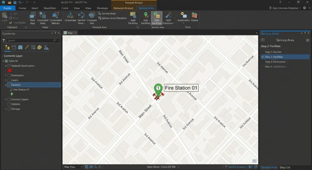 f
Step 3: Set the Break Value
Set the travel-time cutoff to:
10 minutesDepending on the ArcGIS Pro configuration, specify the appropriate time-based break.
The analysis asks:
Which parts of the network can be reached from the facility within 10 minutes?
Step 4: Solve the Service Area
Run the analysis.
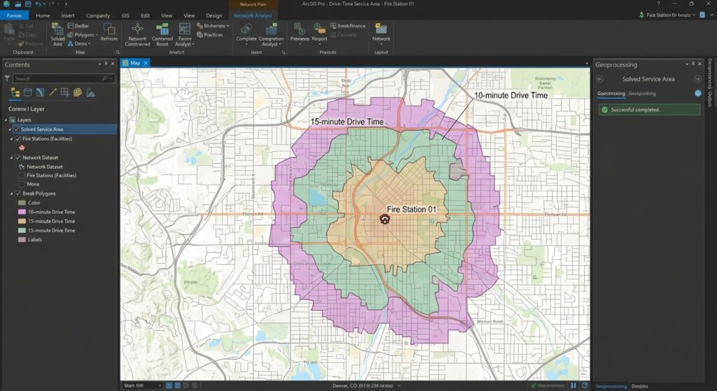
ArcGIS Pro generates a service-area result representing the network-accessible area within the selected travel-time threshold.
Conceptually:
            ┌───────────┐
          ┌─┘           └─┐
        ┌─┘   10-minute   └─┐
       │      service       │
       │       area         │
        └─┐             ┌─┘
          └─────────────┘
                 ●
            Fire Station
The boundary will generally not form a perfect circle because the result follows the transportation network. Unlike standard network analysis in gis shortest path solvers that produce a single line, service areas expand outward across the entire network.
Why Drive-Time Areas Aren’t Circles
A simple Euclidean buffer might produce:
       _______
    .-'       '-.
   /             \
  |      ●        |
   \             /
    '-._______,-'
But a network service area might look more like:
      ────────
     /        \
────●───────────
     \     \
      \─────
          \
The difference occurs because roads determine where travel is actually possible.
A river, railway, one-way street, limited-access highway, or disconnected road can substantially change the accessible area.
Understanding Service Area Output
A service-area result can be used to answer questions such as:
How much of the population is within a 10-minute drive of a hospital?
You can overlay the service area with demographic polygons.
For example:
10-minute service area
          +
Population polygons
          ↓
Population accessible
within 10 minutes
This transforms a network analysis into an accessibility analysis.
Closest Facility GIS Analysis
A related Network Analyst workflow is Closest Facility.
Instead of manually specifying one destination, you can ask:
Which hospital is closest to each incident?
For example:
Emergency Incident
       ↓
Closest Facility Solver
       ↓
Nearest Hospital
       ↓
Travel Time + Distance
This is particularly useful in emergency management.
Example
| Incident | Closest Hospital | Travel Time |
|---|---|---|
| Incident 01 | Hospital A | 7.2 min |
| Incident 02 | Hospital C | 11.5 min |
| Incident 03 | Hospital B | 5.8 min |
Notice that closest should generally be interpreted according to the selected network impedance.
The facility with the shortest geographic distance is not necessarily the facility with the shortest travel time.
Understanding the Dijkstra Algorithm in GIS
Many shortest-path network algorithms are based on graph-search principles. Dijkstra’s algorithm is a classic shortest-path algorithm that determines the minimum-cost path through a weighted network when the relevant edge costs are non-negative.
A simplified network might look like:
      A
     / \
   4/   \7
   /     \
  B---2---C
   \       \
   5\       \3
     \       \
      D---1---E
Each road segment has an associated cost.
The routing algorithm evaluates possible paths and identifies the route with the lowest accumulated cost.
In GIS, however, practical network analysis can involve considerably more than a simple distance-weighted graph. Network datasets may incorporate:
- Travel time
- Direction restrictions
- Turn restrictions
- Barriers
- Road hierarchy
- Time-dependent costs
- Multiple travel modes
Therefore, don’t describe every modern GIS routing result simply as “Dijkstra’s algorithm.” The exact solver and network configuration determine how the analysis is performed.
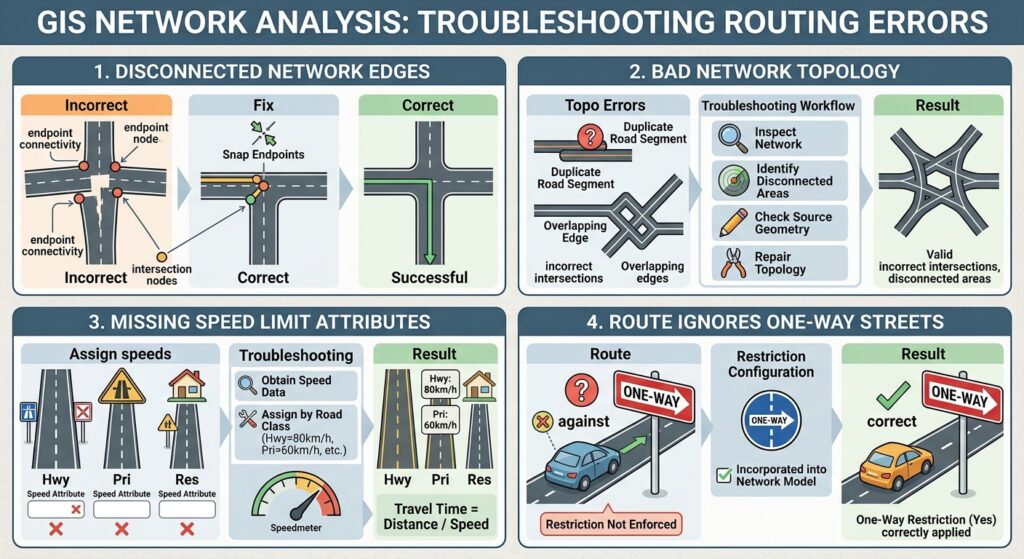
Troubleshooting Network Routing Problems
If you encounter disconnected edges during network analysis in gis shortest path execution, inspect your node snaps and endpoints. Regularly verifying network topology prevents common errors when running a network analysis in gis shortest path solver.
Problem 1: Disconnected Network Edges
Symptom
The solver reports:
- No route found
- Destination unreachable
- Network location cannot be reached
Possible cause
Two roads appear to touch but aren’t actually connected.
For example:
──────────────

       │
       │
       │
The endpoint may be slightly offset from the intersection.
Fix
Inspect the source network data.
Check:
- Endpoint connectivity
- Intersection nodes
- Multipart features
- Gaps between road segments
- Overlapping but unconnected features
Repair the geometry/topology where appropriate and rebuild or update the network dataset.
Problem 2: Bad Network Topology
A network can contain topological inconsistencies such as:
- Duplicate road segments
- Overlapping edges
- Incorrect intersections
- Broken connectivity
- Incorrect elevation/connectivity rules
Troubleshooting workflow
Inspect network
      ↓
Identify disconnected areas
      ↓
Check source geometry
      ↓
Repair topology
      ↓
Rebuild/update network
      ↓
Run route again
Don’t immediately assume that the routing algorithm is wrong. The network source data is often the problem.
Problem 3: Missing Speed Limit Attributes
Accurate speed parameters are vital when performing a network analysis in gis shortest path query that relies on time impedance.
A fastest-route analysis requires a valid travel-time impedance.
If your road data contains:
Road_ID
Length
Road_Type
but no usable speed information, calculating realistic travel time becomes difficult.
A simple conceptual relationship is:
Travel Time = Distance / Speed
For example:
Distance = 10 km
Speed = 50 km/h

Time = 10 / 50 hours
     = 0.2 hours
     = 12 minutes
If speed limits are missing, you may need to:
- Obtain authoritative speed data.
- Assign speeds by road classification.
- Document assumptions.
- Build an appropriate travel-time field.
Example
| Road Type | Assumed Speed |
|---|---|
| Highway | 80 km/h |
| Primary road | 60 km/h |
| Secondary road | 50 km/h |
| Residential road | 30 km/h |
These values are illustrative assumptions, not universal speed limits. For academic analysis, document where your speed values came from.
Problem 4: The Route Ignores One-Way Streets
If a route travels against the direction of a one-way road, check whether the network dataset has a properly configured one-way restriction.
The source data might contain:
One_Way = Yesbut simply having that field does not guarantee that the network solver is using it.
The restriction needs to be incorporated into the network model.
Problem 5: Unrealistic Drive-Time Results
If a 10-minute service area extends an unexpectedly large distance, inspect the travel-time impedance.
Possible causes include:
- Incorrect speed values
- Incorrect units
- Missing travel-time values
- Wrong travel mode
- Incorrect network configuration
For example, accidentally treating:
80 km/has:
80 m/swould produce dramatically incorrect results.
Always verify units.
Network Analysis Quality-Control Checklist
Before submitting a transportation GIS assignment, verify:
Network
- Roads connect correctly.
- Intersections are properly modeled.
- One-way restrictions are configured where relevant.
- Turn restrictions are configured where relevant.
- Network dataset has been built/updated.
Routing
- Origin is correctly located.
- Destination is correctly located.
- Correct travel mode is selected.
- Correct impedance is selected.
- Distance/time units are correct.
Service Area
- Facility is correctly located.
- Break value is appropriate.
- Drive-time impedance is valid.
- Result has been visually inspected.
Documentation
- Network dataset/source documented.
- Speed assumptions documented.
- Impedance documented.
- Analysis date documented if traffic-dependent data is used.
- Limitations discussed.
Shortest Path vs Service Area vs Closest Facility
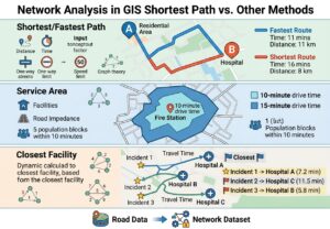
| Analysis | Main Question | Typical Output | Example |
|---|---|---|---|
| Shortest Path | Which route minimizes distance? | Route | Shortest road route between two locations |
| Fastest Path | Which route minimizes travel time? | Route | Fastest ambulance route |
| Service Area | What can be reached within a specified time/distance? | Drive-time polygons/lines | Areas within 10 minutes of a fire station |
| Closest Facility | Which facility can be reached with the lowest network cost? | Routes + facility relationships | Nearest hospital to an emergency |
| Network Dataset | How should the transportation system be modeled? | Routable network | Roads + costs + restrictions |
Final Takeaway
Effective network analysis in GIS shortest path workflows depend on more than simply drawing lines between two points. A reliable transportation analysis requires a properly constructed network dataset with appropriate connectivity, impedance values, and restrictions. Mastering network analysis in gis shortest path workflows allows you to model real-world travel conditions accurately. Mastering network analysis in gis shortest path tools is essential for evaluating urban accessibility and travel efficiency.
 Remember the basic workflow:
Road Data
   ↓
Network Dataset
   ↓
Connectivity + Restrictions + Impedance
   ↓
Network Analyst
   ├── Route → Shortest/Fastest Path
   ├── Service Area → 10-minute Drive-Time Zone
   └── Closest Facility → Nearest Accessible Facility
For university GIS assignments, always explain what you are optimizing—distance, time, or another impedance—and document the assumptions behind your network. A technically correct route solver can still produce misleading results if the underlying road connectivity, speed data, one-way restrictions, or travel-time fields are poorly configured.