
Demystifying Spatial Join & Buffer Analysis in GIS: A Beginner’s Guide
Introduction
Every GIS lab assignment eventually boils down to one of two questions: “What is near this?” and “What overlaps or falls inside this?” Answering the first question is the job of buffer analysis. Answering the second is the job of spatial joins. Together, Spatial Join and Buffer Analysis form the backbone of proximity and overlay analysis in geography, urban planning, and environmental science coursework.
If you’ve ever stared at a shapefile wondering how to figure out which schools sit inside a flood zone, or which crime incidents happened within a certain distance of a bus stop, you were really asking a spatial join and buffer analysis question — you just didn’t have the vocabulary yet. This guide breaks both tools down in plain language, walks through a real lab-style workflow combining them, and flags the mistakes that trip up most first-time GIS students.
By the end, you’ll understand not just how to run these geoprocessing tools in QGIS or ArcGIS, but why each step matters — which is exactly what your instructor is grading you on.
What Is Buffer Analysis?
Before applying Spatial Join and Buffer Analysis together, it helps to understand each tool individually. Buffer analysis is the GIS equivalent of drawing a circle (or a distance-based zone) around a feature to ask, “what falls within this range?” It’s the foundation of proximity analysis in GIS.
A buffer is a polygon generated at a specified distance from a point, line, or polygon feature. There are two common types:
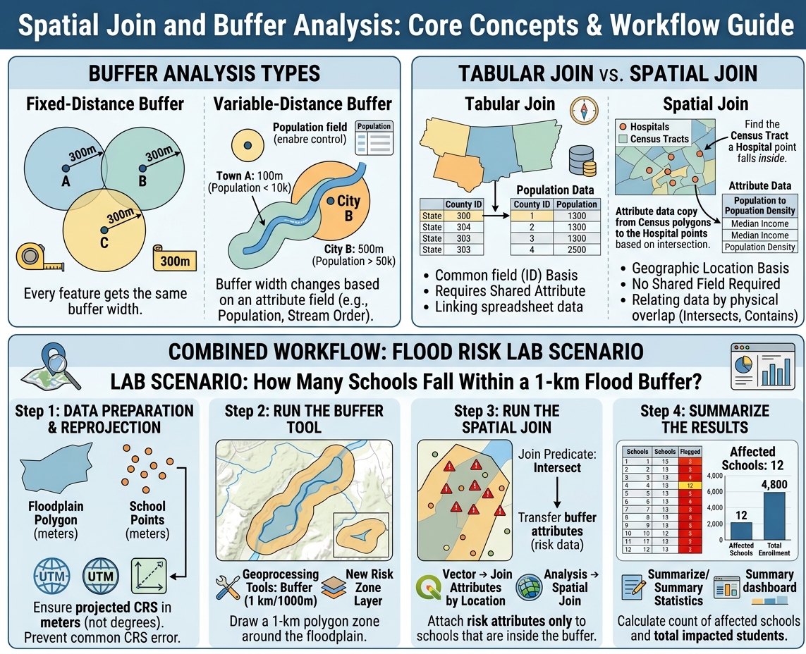
- Fixed-distance buffers — every feature gets the same buffer width. Example: a 500-meter noise buffer around every segment of a highway.
- Variable-distance buffers — the buffer width changes based on an attribute field. Example: larger buffers around major rivers and smaller buffers around minor tributaries, based on stream order.
Common Academic Use Cases
Choosing an appropriate buffer distance is essential when performing Spatial Join and Buffer Analysis for environmental impact studies.
- Noise pollution studies: A 500m buffer around a highway to estimate the population exposed to traffic noise.
- Environmental protection zones: A 30m or 100m buffer around a stream to model riparian protection setbacks.
- Urban planning: A 400m buffer (roughly a 5-minute walk) around transit stops to assess walkability.
- Public health: Buffers around hospitals or clinics to evaluate healthcare accessibility.
Pro Tip: Buffer distance should always match the scale of your research question. A campus-level study might use 50m buffers; a regional environmental study might use 5km buffers. Picking an arbitrary distance without justification is one of the fastest ways to lose marks on a methodology section.
Buffer analysis alone tells you where the zone of influence is. It doesn’t tell you what’s inside it — that’s where spatial joins come in.
What Is a Spatial Join?
A spatial join attaches attribute data from one layer to another based on their location relative to each other, rather than a shared ID or key field. This is the critical difference from a standard tabular join. Unlike attribute joins, a key step in Spatial Join and Buffer Analysis is matching records based purely on geographic location.
Tabular Join vs. Spatial Join
| Feature | Tabular Join | Spatial Join |
|---|---|---|
| Matching basis | Common field (e.g., ID number) | Geographic location |
| Requires shared attribute? | Yes | No |
| Typical use | Joining a spreadsheet to a shapefile’s attribute table | Joining two layers with no shared field |
| Example | Linking population data to counties by FIPS code | Linking census tract demographics to crime points based on which tract each point falls in |
In a spatial join, GIS software checks the geometric relationship between two layers — does a point fall inside a polygon? Does a line intersect a buffer? Is a feature within a certain distance? — and transfers attributes accordingly.
Example: Census Tracts and Crime Data
Imagine you have a point layer of crime incidents and a polygon layer of census tracts with demographic data (income, population density, etc.). Neither layer shares a common ID field. A spatial join lets you ask QGIS or ArcGIS: “for every crime point, find the census tract it physically sits inside, and copy that tract’s attributes onto the point.” Now each crime incident carries median income, population, and other demographic context — without ever touching a shared key field.
This is the essence of a spatial join in QGIS or a spatial join in ArcGIS: relating data by geography, not by ID.
Combining Spatial Join and Buffer Analysis: The Power Workflow
This is where Spatial Join and Buffer Analysis become genuinely powerful — used together, not separately. Most real lab assignments (and real-world consulting projects) require this combination.
Lab Scenario: How Many Schools Fall Within a 1-km Flood Buffer?
Let’s say your assignment is: “Identify all schools within a 1-kilometer buffer of a mapped floodplain, and summarize how many students are potentially affected.”
Here is the exact sequence to follow, using standard geoprocessing tools in GIS:
Step 1: Prepare and Reproject Your Data
Before anything else, confirm your floodplain layer and school points are in a projected coordinate system measured in meters (not a geographic CRS in degrees). This single step prevents the most common error in student labs (more on this below).
Step 2: Run the Buffer Tool
- In QGIS: Vector → Geoprocessing Tools → Buffer. Set distance to 1000 meters.
- In ArcGIS Pro: Analysis → Buffer (or Geoprocessing pane → Buffer). Set distance to 1 kilometer.
This generates a new polygon layer representing the 1-km flood risk zone.
Step 3: Run the Spatial Join (or Intersect)
Now join the school points layer to the buffer polygon:
- In QGIS: Vector → Data Management Tools → Join Attributes by Location.
- In ArcGIS Pro: Analysis → Spatial Join, with school points as the target and the buffer as the join feature, using the “intersect” match option.
This attaches the buffer’s attributes (and confirms which schools fall inside it) to each school point.
Pro Tip: When your goal is simply “does it fall inside,” use the Intersect predicate. Use “within a distance” instead when you want to catch features that are close but don’t technically touch the buffer boundary.
Step 4: Summarize the Results
Once joined, open the attribute table and use Summarize (QGIS) or Summary Statistics (ArcGIS) to count how many school records fall inside the buffer, and total up enrollment figures if that field exists.
The sequence — Buffer → Spatial Join/Intersect → Summarize — is the standard workflow pattern for nearly every proximity-based GIS assignment, whether you’re studying flood risk, noise exposure, or service area coverage.
Troubleshooting Common Student Errors
A frequent mistake during Spatial Join and Buffer Analysis is buffering features in a geographic coordinate system (degrees) rather than a projected system (meters). Even with the right workflow, small setup mistakes derail most lab results. Here are the errors instructors see most often:
- Buffering in a geographic CRS (degrees) instead of a projected CRS (meters/feet). A “1000” buffer in WGS84 creates a buffer 1000 degrees wide — essentially covering the globe. Always reproject to a local projected CRS (like UTM) before buffering.
- Using the wrong join type: one-to-one vs. one-to-many. If multiple buffer polygons overlap a single point, a one-to-one join will only keep one match, silently dropping data. Choose “one-to-many” (or “join all matching features”) in ArcGIS, or use the appropriate summary option in QGIS, when overlapping zones are expected.
- Forgetting to check the join predicate. “Intersects,” “within,” “contains,” and “closest” all behave differently. Selecting the wrong one produces a join that runs without errors but returns incorrect matches.
- Mismatched coordinate systems between layers. If your school points and buffer layer use different CRSs, the spatial join can fail silently or return zero matches. Always confirm both layers share the same projection before joining.
- Not validating results with a quick visual check. Before writing up findings, symbolize the joined layer and visually confirm that flagged features actually sit where you expect them to on the map.
Pro Tip: If your spatial join returns zero results and you’re confident the geography is correct, the first thing to check is always the coordinate reference system — mismatched CRSs cause more silent failures than any other single issue in GIS coursework.
Conclusion: Master Spatial Join and Buffer Analysis
Mastering Spatial Join and Buffer Analysis gives you the two most-used geoprocessing tools in the entire GIS toolkit. Once you’re comfortable running buffers to define zones of influence and spatial joins to relate features by location rather than shared keys, you’re equipped to tackle far more advanced spatial modeling — from suitability analysis to network-based accessibility studies to environmental impact assessments.
These two tools aren’t just lab exercises to check off — they’re the analytical foundation that every advanced GIS technique in your degree builds on. Get comfortable with the Buffer → Spatial Join → Summarize sequence now, and every future geoprocessing assignment gets noticeably easier.
If your coursework moves into more complex geoprocessing — multi-criteria overlay analysis, network analysis, or custom Python scripting with PyQGIS or ArcPy — consider reaching out to your department’s GIS lab support or a tutoring resource for hands-on guidance. Complex spatial modeling is far easier to learn with feedback on your actual workflow than from a textbook alone.