Table of Contents

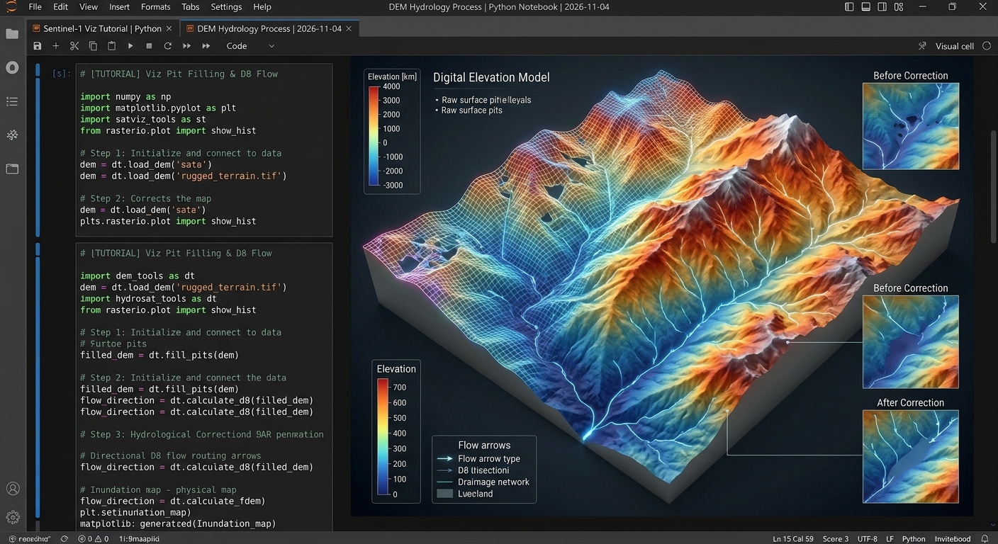
Automated Watershed Delineation and Stream Network Extraction Using PySheds and DEMs

Automated watershed modeling is a foundational pillar of modern hydro-environmental engineering. Whether managing regional water resources, evaluating urban flood risks, or planning ecological conservation reserves, spatial analysts and hydrologists rely heavily on Digital Elevation Models (DEMs) to reconstruct surface drainage topologies. Traditionally, extracting catchments and stream networks required tedious point-and-click operations within closed-source desktop geographic information systems (GIS).

Today, leveraging the Automated Watershed Delineation PySheds DEM Python ecosystem allows engineers to script, scale, and automate entire hydrological pipelines. This tutorial provides a comprehensive, production-grade guide to ingesting raster elevations, conditioning surfaces, routing surface water via the D8 algorithm, generating accumulation maps, and delineating precise catchment boundaries using Python and PySheds.

Introduction: The Imperative of Automated Hydrological Modeling

Hydrological simulation models require accurate topological representations of the Earth’s surface to determine how precipitation travels across a watershed. When rain falls over complex topography, gravity dictates overland flow paths from high-elevation ridges down into tributary streams, major rivers, and outlet pour points.

Manual delineation of these basins is impractical for large regional catchments. By automating the extraction of river networks and catchment polygons in Python, engineers can rapidly iterate through different climate scenarios, integrate real-time telemetry, and scale models across national boundaries. Advanced terrain processing also unlocks downstream capabilities, such as pairing topographic analysis with 3D Solar Radiation Modeling on Complex Terrain to evaluate microclimate evaporation rates, or feeding basin discharge estimates into Sentinel-1 SAR Flood Mapping pipelines during emergency response operations.

Core Hydrological Processing Pipeline

Before diving into code, it is essential to understand the theoretical stages required to transform raw elevation rasters into clean drainage networks:

DEM Conditioning & Sink Filling: Raw DEMs invariably contain data errors, pits, and artificial depressions (sinks) where water would become trapped indefinitely. Conditioning involves identifying these anomalies and raising their elevation values to ensure continuous hydrologic connectivity.
Flow Direction Routing: Using the conditioned elevation grid, the algorithm determines the steepest descent direction for every pixel. The standard D8 routing scheme assigns flow from each cell to one of its eight immediate horizontal, vertical, or diagonal neighbors.
Flow Accumulation Computation: By tracing flow direction paths downstream, the model calculates the cumulative number of upstream cells that drain through each individual pixel. High accumulation values designate valleys and stream channels, while low values represent ridge tops.
Catchment Delineation: By selecting an outlet coordinate (pour point), snapping it to the nearest high-accumulation stream cell, and tracing all contributing upstream pixels, the algorithm isolates the exact bounding polygon of the watershed.

Step-by-Step Automated Watershed Delineation PySheds DEM Python Implementation

To execute this pipeline, ensure your Python environment includes pysheds, rasterio, numpy, matplotlib, and geopandas.

1. Ingesting Elevation Raster Grids and Defining Spatial Reference Systems

When initializing Automated Watershed Delineation PySheds DEM Python scripts, the initial step involves loading a raster DEM file (such as a GeoTIFF) into memory via PySheds' Grid interface. This preserves coordinate reference systems (CRS), affine transformation matrices, and bounding box extents.

Python

import numpy as np
import matplotlib.pyplot as plt
from matplotlib.colors import LogNorm
from pysheds.grid import Grid

# Initialize grid from DEM raster
dem_path = "data/regional_dem.tif"
grid = Grid.from_raster(dem_path)

# Read elevation data into a NumPy array
dem = grid.read_raster(dem_path)

print(f"Raster Dimensions: {dem.shape}")
print(f"Spatial Reference System (CRS): {grid.crs}")
print(f"Affine Transform: {grid.affine}")

# Visualize raw DEM
fig, ax = plt.subplots(figsize=(8, 6))
im = ax.imshow(dem, cmap='terrain', extent=grid.extent)
plt.colorbar(im, ax=ax, label='Elevation (meters)')
plt.title('Raw Digital Elevation Model (DEM)')
plt.xlabel('Easting')
plt.ylabel('Northing')
plt.show()

2. Resolving DEM Depressions and Calculating Flow Routing Arrays

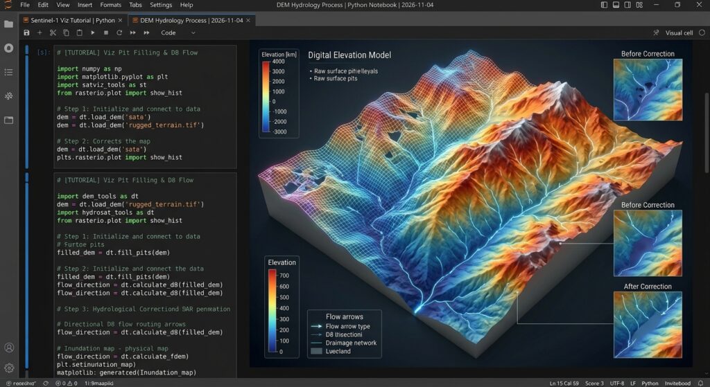
DEM conditioning and flow direction routing steps in Automated Watershed Delineation PySheds DEM Python workflows.

When executing Automated Watershed Delineation PySheds DEM Python workflows, ensuring that flat terrain gradients are properly resolved is critical before calculating flow direction arrays. Proper surface conditioning is a vital prerequisite for any robust Automated Watershed Delineation PySheds DEM Python pipeline. Raw elevation models contain surface sinks that impede flow routing. We apply a three-stage conditioning sequence: filling single-cell pits, flooding multi-cell depressions, and resolving flat zones where slope gradients drop to zero. Following conditioning, we compute the D8 flow direction matrix.

Python

# Step 2.1: Fill single-cell pits
pit_filled_dem = grid.fill_pits(dem)

# Step 2.2: Fill broader multi-cell depressions
flooded_dem = grid.fill_depressions(pit_filled_dem)

# Step 2.3: Resolve flat areas to ensure continuous drainage gradients
conditioned_dem = grid.resolve_flats(flooded_dem)

# Define standard D8 dirmap (ESRI convention)
# North: 64, NE: 128, East: 1, SE: 2, South: 4, SW: 8, West: 16, NW: 32
dirmap = (64, 128, 1, 2, 4, 8, 16, 32)

# Calculate D8 flow direction grid
fdir = grid.flowdir(conditioned_dem, dirmap=dirmap)

print("Flow direction routing array computed successfully.")

3. Generating Flow Accumulation Grids and Extracting Stream Networks

Once flow directions are established, computing flow accumulation reveals the drainage network structure. By applying a threshold to the accumulation array, we isolate stream channels.

Leveraging Automated Watershed Delineation PySheds DEM Python scripts to compute upstream drainage cells enables automated channel extraction across complex topographies.

Python

# Calculate accumulated number of upstream cells for every pixel
acc = grid.accumulation(fdir, dirmap=dirmap)

# Visualize flow accumulation on a logarithmic scale
fig, ax = plt.subplots(figsize=(8, 6))
im = ax.imshow(acc, extent=grid.extent, cmap='cubehelix', norm=LogNorm(1, acc.max()))
plt.colorbar(im, ax=ax, label='Upstream Drainage Cells')
plt.title('Flow Accumulation Surface')
plt.xlabel('Easting')
plt.ylabel('Northing')
plt.show()

# Extract stream network using an accumulation threshold (e.g., >= 1000 contributing cells)
stream_threshold = 1000
streams = acc > stream_threshold

# Visualize extracted streams
fig, ax = plt.subplots(figsize=(8, 6))
ax.imshow(streams, extent=grid.extent, cmap='bone')
plt.title(f'Extracted Stream Network (Threshold > {stream_threshold} cells)')
plt.xlabel('Easting')
plt.ylabel('Northing')
plt.show()

4. Specifying Pour Points and Delineating Upstream Catchment Boundaries

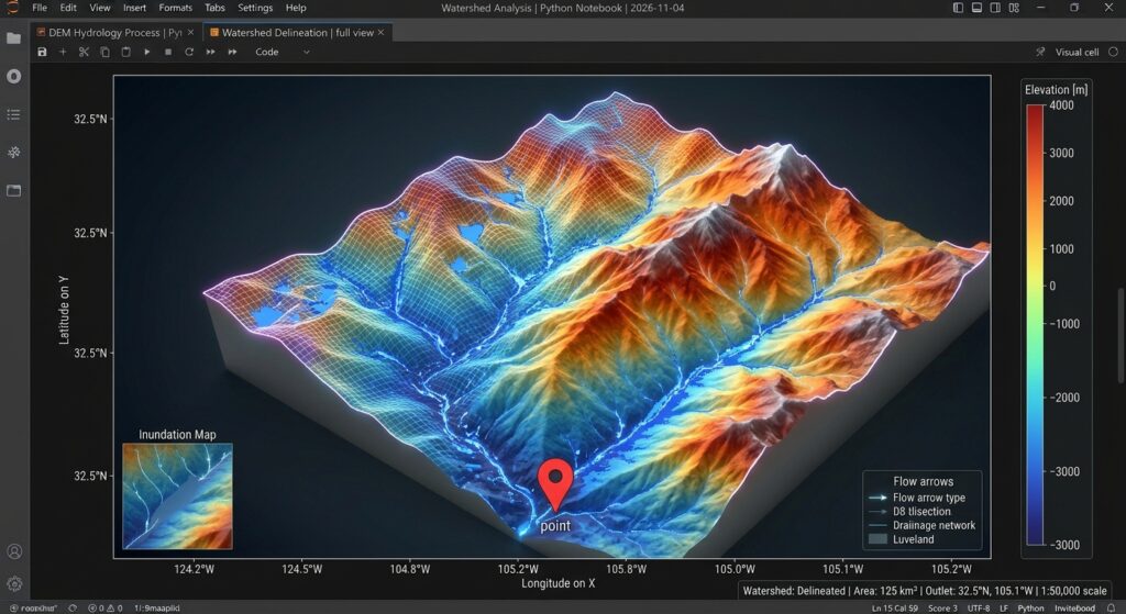
To isolate a specific watershed basin, we define a downstream outlet (pour point). Because raw coordinates may fall slightly off the exact stream channel, PySheds provides a snapping utility to anchor the pour point to the nearest high-accumulation pixel.

Python

# Define approximate outlet coordinate (X, Y in projection CRS)
outlet_x, outlet_y = 375200.0, 9821000.0

# Snap pour point to the highest accumulation cell within a local search radius
# Ensuring it lies directly on our extracted stream network (acc > 1000)
x_snap, y_snap = grid.snap_to_mask(acc > 1000, (outlet_x, outlet_y))

print(f"Original Outlet: ({outlet_x}, {outlet_y})")
print(f"Snapped Pour Point: ({x_snap}, {y_snap})")

# Delineate the upstream catchment boundary
catchment = grid.catchment(
    x=x_snap, 
    y=y_snap, 
    fdir=fdir, 
    dirmap=dirmap, 
    xytype='coordinate'
)

# Clip the grid view to the delineated catchment bounding box
grid.clip_to(catchment)
clipped_catchment = grid.view(catchment)
clipped_acc = grid.view(acc)

# Plot the final delineated watershed and stream network
fig, ax = plt.subplots(figsize=(8, 6))
im = ax.imshow(
    np.where(clipped_catchment, clipped_acc, np.nan),
    extent=grid.extent,
    cmap='cubehelix',
    norm=LogNorm(1, clipped_acc.max()),
    interpolation='bilinear'
)
plt.colorbar(im, ax=ax, label='Upstream Contributing Cells')
plt.scatter([x_snap], [y_snap], color='red', s=60, marker='o', label='Outlet Pour Point')
plt.legend(loc='upper right')
plt.title('Delineated Watershed Catchment Basin')
plt.xlabel('Easting')
plt.ylabel('Northing')
plt.show()

Exporting Vectors for Downstream GIS Analysis

To convert raster catchment masks into vector polygons for integration into GeoPandas vector workflows, utilize rasterio.features.shapes:

Python

import geopandas as gpd
from rasterio.features import shapes
from shapely.geometry import shape

# Generate polygon shapes from catchment mask
shape_generator = shapes(
    clipped_catchment.astype(np.uint8), 
    transform=grid.affine
)

records = []
for geom, val in shape_generator:
    if val == 1:
        records.append({
            "type": "Feature",
            "geometry": geom,
            "properties": {"basin_id": 1}
        })

if records:
    watershed_gdf = gpd.GeoDataFrame.from_features(records, crs=grid.crs)
    watershed_gdf.to_file("delineated_watershed.geojson", driver="GeoJSON")
    print("Successfully exported watershed boundary to delineated_watershed.geojson")

Conclusion

Automating hydrological workflows with Python and PySheds removes the friction of manual desktop GIS processing, enabling robust, reproducible watershed delineation and stream network extraction. By executing rigorous DEM conditioning, D8 flow routing, accumulation thresholding, and coordinate snapping, data scientists and water resource engineers can seamlessly scale catchment analysis across arbitrary geographic extents. Ultimately, mastering Automated Watershed Delineation PySheds DEM Python pipelines empowers engineers to replace tedious desktop GIS tasks with rapid, scalable Python automation.

Want to master advanced spatial workflows? Bookmark this guide on Automated Watershed Delineation PySheds DEM Python, or reach out to our team if you need expert professional assistance with your advanced GIS assignments.