
Processing Sentinel-1 Synthetic Aperture Radar (SAR) Data for Flood Inundation Mapping in Python
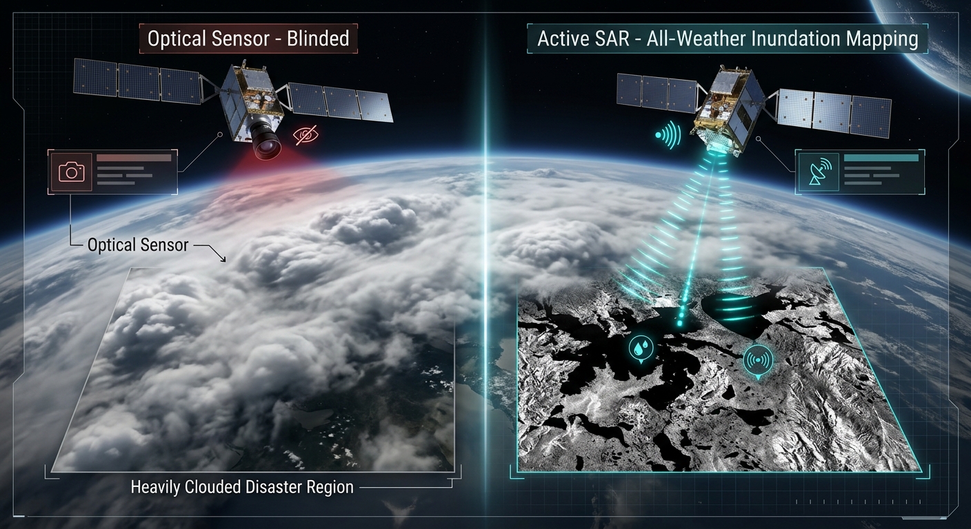
During extreme hydro-meteorological emergencies and riverine overflow events, optical satellite constellations (such as Sentinel-2 or Landsat) are frequently rendered blind. Persistent heavy cloud cover, dense atmospheric moisture, and torrential precipitation obscure the ground surface precisely when disaster response teams require high-resolution situational awareness.
To bypass atmospheric interference, remote sensing hydrologists rely on active microwave imaging systems. Sentinel-1 SAR Flood Inundation Mapping Python pipelines provide an operational framework to capture ground conditions day or night, regardless of weather.
This applied technical tutorial covers the theoretical principles of radar backscatter, the end-to-end processing of Sentinel-1 Ground Range Detected (GRD) scenes using Python, and the extraction of reliable flood inundation layers via change detection, Otsu thresholding, and permanent water masking.
Introduction: The Power of Microwave Remote Sensing in Flood Disasters
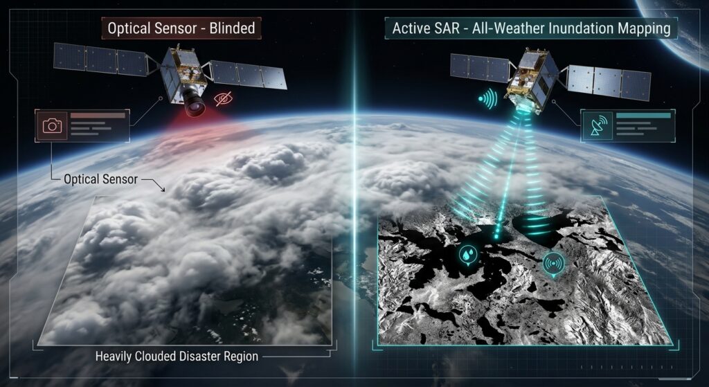
Optical sensors capture passive solar radiation reflected from the Earth’s surface within visible and infrared wavelengths. When major floods occur, storm systems blanket disaster areas in thick cloud shields, rendering optical imagery useless.
Synthetic Aperture Radar (SAR) systems operate differently. Operating in the C-band (~5.4 GHz frequency, ~5.6 cm wavelength), SAR is an active sensor that transmits its own microwave pulses toward the Earth and measures the returning backscattered signal intensity. Because microwaves pass seamlessly through clouds, smoke, and heavy rain, SAR guarantees data acquisition during critical disaster windows.
Technical Principles of SAR: Specular vs. Diffuse Scattering
When studying radar backscatter for Sentinel-1 SAR flood inundation mapping Python applications, understanding how microwaves interact with different surfaces is essential. Mapping floods with SAR relies fundamentally on measuring changes in radar backscatter intensity, expressed in decibels ($\text{dB}$). Different land cover types interact uniquely with C-band microwaves:
-
Rough Surfaces and Vegetation (High Backscatter): Natural land covers, dense vegetation, urban structures, and rough soil create diffuse scattering. Incident radar waves bounce randomly in multiple directions, sending a significant portion of energy back to the satellite antenna. This yields bright pixels in the SAR image.
-
Standing Water (Low Backscatter): Calm or slowly moving floodwaters act as a flat specular reflector. When radar pulses strike smooth standing water at an oblique angle, the energy is reflected forward away from the sensor (like a mirror). Very little backscatter returns to the satellite, producing exceptionally dark, low-intensity pixel values.
By comparing pre-flood baseline scenes with post-flood observations, GIS analysts isolate these low backscatter anomalies to delineate flood boundaries.
Step-by-Step Sentinel-1 SAR Flood Inundation Mapping Python Workflow
Implementing an automated radar processing chain requires handling spatial metadata, calibrating raw pixel digital numbers (DN) into physical backscatter coefficients, filtering speckle noise, and executing threshold-based binarization.
1. Accessing Pre- and Post-Flood Sentinel-1 GRD Scenes
To acquire data programmatically, developers often interface with cloud archives or STAC catalogs. For seamless query parameters and search workflows across cloud-native spatiotemporal asset catalogues, you can integrate STAC API satellite data pipelines to pull Sentinel-1 GRD scenes.
2. Executing Radiometric Calibration, Speckle Filtering, and Terrain Correction
When executing Sentinel-1 SAR flood inundation mapping Python pipelines, raw Sentinel-1 images must be radiometrically calibrated to $\sigma^\circ$ (sigma nought), filtered to remove inherent granular speckle noise (using Lee or Gamma filters), and terrain-corrected to remove geometric distortions caused by topography.
We can automate these routines using
pyroSAR and rasterio. For complementary vector operations and geographic visualization workflows, see our guide on QGIS raster processing automation.Python
import os
import numpy as np
import rasterio
from rasterio.plot import show
from scipy.ndimage import median_filter
import matplotlib.pyplot as plt

def load_and_preprocess_sar(image_path):
    """
    Loads a preprocessed Sentinel-1 SAR GeoTIFF slice
    and applies secondary spatial filtering for flood analysis.
    """
    with rasterio.open(image_path) as src:
        meta = src.meta.copy()
        # Read VV polarization band (standard for flood mapping)
        sar_data = src.read(1).astype(np.float32)
        transform = src.transform
        crs = src.crs

    # Convert DN to decibels if not already scaled: dB = 10 * log10(intensity)
    # Assuming input is linear power, convert safely
    with np.errstate(divide='ignore', invalid='ignore'):
        sar_db = 10.0 * np.log10(sar_data)
        sar_db[np.isinf(sar_db)] = np.nan

    # Apply a median filter to suppress remaining speckle texture
    filtered_db = median_filter(np.nan_to_num(sar_db, nan=0.0), size=5)

    return filtered_db, meta, transform, crs

# Example invocation path placeholders
# pre_path = "data/sentinel1_pre_flood.tif"
# post_path = "data/sentinel1_post_flood.tif"
3. Applying Change Detection and Otsu Thresholding
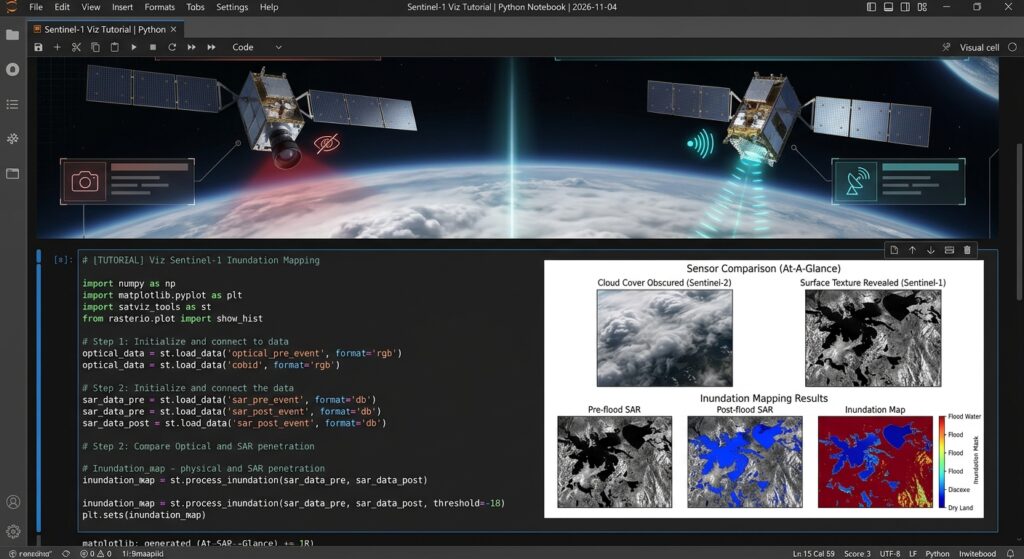
To extract standing water extent masks during automated Sentinel-1 SAR flood inundation mapping Python routines, we implement a change detection approach combined with automated thresholding. Otsu’s thresholding algorithm computes an optimal separation boundary between dry land and water classes in the bimodal backscatter histogram.
Automating the binarization step is critical for scalable Sentinel-1 SAR flood inundation mapping Python workflows.
from skimage.filters import threshold_otsu

def extract_flood_extent(pre_db, post_db, threshold_offset=-3.0):
    """
    Performs change detection between pre- and post-flood SAR imagery
    and applies Otsu thresholding to isolate flooded pixels.
    """
    # Calculate backscatter difference (Post - Pre)
    # Significant drops in dB indicate newly emerged water surfaces
    diff_image = post_db - pre_db

    # Valid pixels only
    valid_mask = ~np.isnan(diff_image) & (post_db != 0)
    valid_diff = diff_image[valid_mask]

    if valid_diff.size == 0:
        raise ValueError("No valid overlapping pixels found in SAR rasters.")

    # Calculate automated threshold using scikit-image Otsu method
    try:
        thresh = threshold_otsu(valid_diff)
    except Exception:
        thresh = -3.0 # Fallback empirical threshold

    print(f"Calculated optimal change detection threshold: {thresh:.2f} dB")

    # Binary classification: areas with drop greater than threshold are potential floods
    flood_mask = np.zeros_input = np.zeros(diff_image.shape, dtype=np.uint8)
    flood_mask[(diff_image <= thresh) & valid_mask] = 1

    return flood_mask, diff_image
4. Masking Permanent Water Bodies
A common artifact in radar flood mapping is the false classification of permanent water bodies (rivers, lakes, reservoirs) as “new flood zones.” To isolate true temporary inundation, we subtract an authoritative permanent water mask (such as the JRC Global Surface Water dataset or ESA GlobCover). For hydrological routing and upstream basin context prior to masking, refer to our tutorial on Automated Watershed Delineation in Python.
Python
def mask_permanent_water(flood_mask, permanent_water_raster_path):
    """
    Removes permanent water bodies from the candidate flood mask
    to retain strictly temporary flood inundation zones.
    """
    with rasterio.open(permanent_water_raster_path) as perm_src:
        perm_water = perm_src.read(1)

    # Ensure binary mask format (1 = permanent water, 0 = land)
    perm_water_binary = np.where(perm_water > 0, 1, 0)

    # Exclude permanent water from the dynamic flood mask
    isolated_flood_mask = np.where((flood_mask == 1) & (perm_water_binary == 0), 1, 0)

    return isolated_flood_mask

def export_flood_vector(flood_mask, transform, crs, output_geojson_path):
    """
    Vectorizes the raster flood inundation mask into standard GeoJSON polygons.
    """
    import geopandas as gpd
    from rasterio.features import shapes

    shape_generator = shapes(
        flood_mask.astype(np.uint8),
        mask=(flood_mask == 1),
        transform=transform
    )

    records = []
    for geom, value in shape_generator:
        records.append({
            "type": "Feature",
            "geometry": geom,
            "properties": {"grid_code": int(value)}
        })

    if records:
        gdf = gpd.GeoDataFrame.from_features(records, crs=crs)
        gdf.to_file(output_geojson_path, driver="GeoJSON")
        print(f"Successfully exported flood polygons to {output_geojson_path}")
    else:
        print("No flood features detected above threshold.")
Visualizing Results
Summary
Processing Sentinel-1 Synthetic Aperture Radar data in Python provides disaster management teams with a reliable, all-weather capability to map flood dynamics. By executing precise radiometric preparation, change detection analysis, automated Otsu thresholding, and permanent water masking via
rasterio and scientific Python libraries, GIS analysts can rapidly transform raw satellite telemetry into actionable vector intelligence.Want to master advanced remote sensing workflows? Bookmark this guide on Sentinel-1 SAR flood inundation mapping Python, or reach out to our team if you need professional assistance with your advanced GIS assignments.
Want to master advanced remote sensing workflows? Bookmark this guide on Sentinel-1 SAR flood inundation mapping Python, or reach out to our team if you need professional assistance with your advanced GIS assignments.