
Spatial Autocorrelation in Practice: Calculating Global and Local Moran’s I for Disease Cluster Analysis

In epidemiological surveillance and public health spatial analytics, traditional aspatial statistical models frequently fall short. Standard regression techniques assume that observations are independent and identically distributed (i.i.d.). However, health outcomes, infectious disease transmissions, chronic morbidity rates, and environmental toxic exposures rarely adhere to independence across space.
This spatial dependence is formally captured by Tobler’s First Law of Geography: “Everything is related to everything else, but near things are more related than distant things.”
When disease rates cluster geographically—whether due to shared environmental contaminants, vector habitats, socioeconomic disparities, or clustered person-to-person transmission—ignoring spatial structure leads to biased parameter estimates, inflated Type I error rates, and flawed public health interventions. This analytical guide explores the theoretical foundations and hands-on Python implementation of spatial autocorrelation metrics using PySAL and GeoPandas, focusing specifically on Global Moran’s I and Local Indicators of Spatial Association (LISA) / Anselin Local Moran’s I for robust disease cluster analysis.
Methodology Overview: Global vs. Local Spatial Autocorrelation
To rigorously evaluate how disease rates distribute across geographic space, quantitative epidemiologists rely on two complementary classes of spatial autocorrelation statistics: Global and Local measures.
1. Global Moran’s I: Assessing Overall Spatial Pattern
Global Moran’s I evaluates the entire study area to determine whether the spatial pattern of a health variable (e.g., standardized incidence ratios or disease mortality rates) exhibits clustering, dispersion, or spatial randomness.
Mathematically, Global Moran’s I is expressed as:
$$I = \frac{N}{S_0} \sum_{i=1}^{N} \sum_{j=1}^{N} w_{ij} (x_i – \bar{x})(x_j – \bar{x}) \Big/ \sum_{i=1}^{N} (x_i – \bar{x})^2$$
Where:
-
$N$ is the total number of spatial units (e.g., census tracts, counties, health districts).
-
$x_i$ and $x_j$ represent the attribute values (disease incidence) at locations $i$ and $j$.
-
$\bar{x}$ is the mean of the attribute across all locations.
-
$w_{ij}$ is the spatial weight defining the neighborhood relationship between feature $i$ and feature $j$.
-
$S_0$ is the sum of all spatial weights: $S_0 = \sum_{i=1}^{N} \sum_{j=1}^{N} w_{ij}$.
Interpretation:
-
$I > 0$: Positive spatial autocorrelation (similar values cluster together, such as high disease rates adjacent to high rates).
-
$I < 0$: Negative spatial autocorrelation (checkerboard pattern where high values are surrounded by low values).
-
$I \approx 0$: Spatial randomness.
While Global Moran’s I provides a single summary statistic of global spatial structure, it masks local heterogeneity. A region can have an overall random global statistic while harboring significant localized disease outbreaks.
2. Local Moran’s I (Anselin LISA)
To pinpoint precise disease clusters, Anselin introduced Local Indicators of Spatial Association (LISA). Local Moran’s I decomposes the global index into individual spatial components for each areal unit $i$:
$$I_i = \frac{x_i – \bar{x}}{m_2} \sum_{j=1}^{N} w_{ij} (x_j – \bar{x})$$
Where $m_2 = \frac{\sum_{i=1}^{N} (x_i – \bar{x})^2}{N}$.
LISA statistics evaluate statistical significance against a spatial randomness reference distribution generated via conditional permutation (Monte Carlo simulation). The resulting local statistics classify each spatial unit into one of four distinct quadrant categories on a Moran Scatterplot:
-
High-High (Hot Spots): High disease rates surrounded by neighboring units with high disease rates. Represents primary public health intervention priorities.
-
Low-Low (Cold Spots): Low disease rates surrounded by low-rate neighbors. Indicates protected or low-risk zones.
-
High-Low (Spatial Outlier): High disease incidence surrounded by low-rate neighbors. May point to localized environmental point sources, occupational hazards, or reporting anomalies.
-
Low-High (Spatial Outlier): Low disease incidence surrounded by high-rate neighbors. Indicates protected pockets within high-risk endemic areas.
Step-by-Step Python Implementation (PySAL & GeoPandas)
Conducting advanced spatial autocorrelation analysis requires specialized spatial libraries in Python. We will use
geopandas for vector data manipulation, libpysal for constructing spatial weight matrices, and esda for executing Global and Local Moran’s I calculations.Step 1: Constructing Spatial Weight Matrices
Spatial weights ($W$) formalize the geographic relationship between spatial features. Choosing the appropriate weighting scheme—such as Queen contiguity, Rook contiguity, or $k$-nearest neighbors ($k$-NN)—directly impacts analytical outcomes.
Python
import geopandas as gpd
import libpysal
import numpy as np
import pandas as pd
import matplotlib.pyplot as plt
import esda
from splot.esda import plot_moran, lisa_cluster

# Load disease incidence shapefile (e.g., county-level cholera or malaria incidence)
gdf = gpd.read_file("path/to/disease_incidence_data.shp")

# 1. Queen Contiguity Weights (shares common edge or vertex)
w_queen = libpysal.weights.Queen.from_dataframe(gdf, use_index=True)

# 2. Rook Contiguity Weights (shares common edge only)
w_rook = libpysal.weights.Rook.from_dataframe(gdf, use_index=True)

# 3. K-Nearest Neighbors Weights (e.g., 5 nearest centroid neighbors)
# Useful for handling irregular polygon sizes or isolated rural districts
w_knn = libpysal.weights.KNN.from_dataframe(gdf, k=5, use_index=True)

# Row-standardize weights so that rows sum to 1 (essential for smoothing variance)
w_queen.transform = 'R'

print(f"Number of observations: {len(gdf)}")
print(f"Average number of neighbors (Queen): {w_queen.mean_neighbors:.2f}")
Step 2: Calculating Global Moran’s I Test Statistics
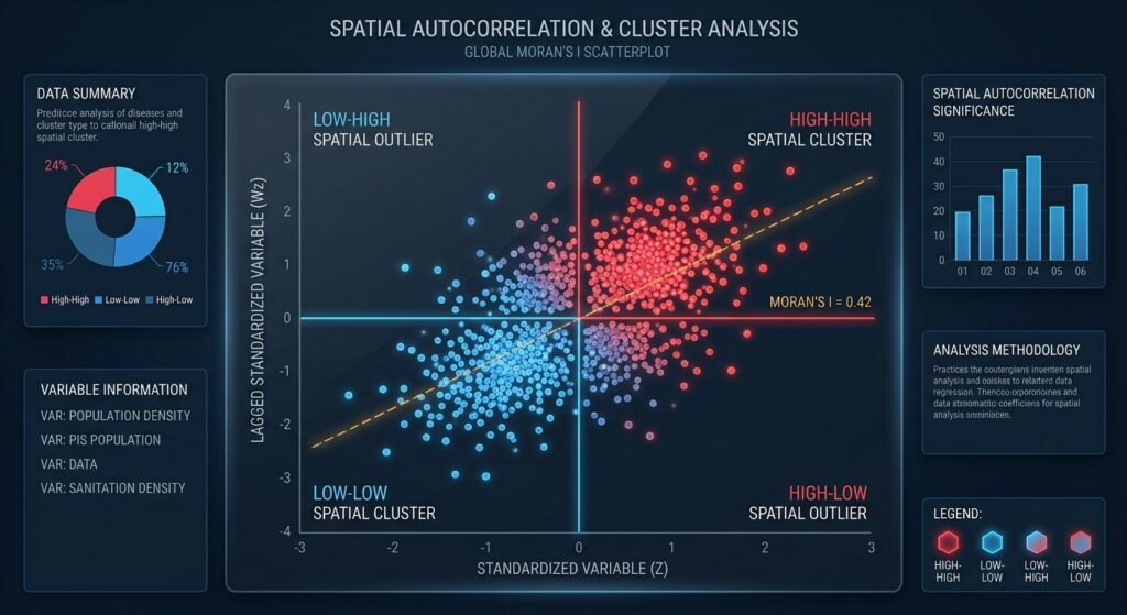
Once the spatial weights matrix is row-standardized, we calculate Global Moran’s I for our target epidemiological variable (e.g.,
incidence_rate).Python
# Extract target attribute series
y = gdf['incidence_rate'].values

# Calculate Global Moran's I with permutation-based inference (999 simulations)
mi = esda.moran.Moran(y, w_queen, permutations=999)

print(f"Global Moran's I Statistic: {mi.I:.4f}")
print(f"Expected Value under Null Hypothesis: {mi.EI:.4f}")
print(f"Pseudo p-value: {mi.p_sim:.4f}")
print(f"Z-score: {mi.z_sim:.4f}")

# Visualize Moran Scatterplot
fig, ax = plot_moran(mi, zstandard=True, figsize=(6, 6))
plt.title("Global Moran Scatterplot: Disease Incidence Rate", fontsize=12)
plt.xlabel("Standardized Incidence Rate")
plt.ylabel("Spatial Lag of Incidence Rate")
plt.show()
If the pseudo p-value is less than the standard significance threshold ($p < 0.05$) and the z-score is positive, we reject the null hypothesis of spatial randomness and confirm significant global spatial clustering across the study region.
Step 3: Generating Local Indicators of Spatial Association (LISA)
To isolate localized hot spots and spatial outliers, we execute Anselin Local Moran’s I using
esda.Moran_Local.Python
# Compute Local Moran's I with 999 permutations for robust pseudo p-values
lm = esda.moran.Moran_Local(y, w_queen, permutations=999)

# Assign local statistics back to the GeoDataFrame
gdf['local_i'] = lm.Is
gdf['p_value'] = lm.p_sim
gdf['quadrant'] = lm.q

# Print summary counts per quadrant
quadrant_labels = {1: 'High-High', 2: 'Low-High', 3: 'Low-Low', 4: 'High-Low'}
gdf['quad_label'] = gdf['quadrant'].map(quadrant_labels)
print(gdf['quad_label'].value_counts())
Step 4: Visualizing and Interpreting LISA Cluster Maps
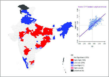
To make these analytical outputs actionable for healthcare administrators, we map statistically significant local clusters. Standard practice filters out units where the pseudo p-value exceeds $0.05$ (classifying them as “Not Significant”).
Python
# Create significance mask (p < 0.05)
significance_mask = gdf['p_value'] < 0.05

# Plot LISA Cluster Map using splot
fig, ax = plt.subplots(figsize=(10, 10))
lisa_cluster(lm, gdf, p=0.05, ax=ax)
plt.title("LISA Cluster Map: Local Disease Hot Spots & Outliers (p < 0.05)", fontsize=14)
plt.axis('off')
plt.show()
Public Health Intervention Planning & Spatial Interpretation
Translating statistical output into clinical and logistical interventions requires rigorous quadrant interpretation:
-
High-High Clusters (Target Hot Spots): These zones represent contiguous regions experiencing elevated disease burdens. Public health agencies must deploy immediate resources here: mobile vaccination clinics, targeted vector control (e.g., indoor residual spraying for malaria), or emergency water purification infrastructure in waterborne outbreak scenarios. For broader contextual understanding of service accessibility, analysts frequently cross-reference these findings with healthcare desert spatial mismatch analysis.
-
Low-Low Clusters (Protected Areas): These regions act as protective benchmarks. Epidemiologists should investigate what socio-environmental factors (e.g., robust sanitation, high socioeconomic status, effective primary healthcare coverage) maintain low transmission rates.
-
High-Low Outliers (Isolated Outbreaks): A high-rate district surrounded by low-rate neighbors. This pattern often signals localized institutional failure—such as a failing wastewater treatment plant, a contaminated municipal well, or a localized hospital-acquired outbreak. Analysts investigating localized event density can pair these insights with crime density KDE analysis or spatial point pattern tutorials to pinpoint exact coordinate-level clustering.
-
Low-High Outliers (Vulnerable Buffers): Low-rate districts directly exposed to high-incidence neighbors. These areas face immediate contagion spillover risk and require aggressive preventive screening and prophylactic distribution.
Methodological Considerations & Analytical Pitfalls
When deploying spatial autocorrelation in epidemiological research, analysts must navigate several methodological challenges:
-
Modifiable Areal Unit Problem (MAUP): Spatial statistics are highly sensitive to the scale and aggregation zones of spatial units (e.g., shifting from county-level to census-block-level analysis changes neighborhood adjacency structures). Always report scale dependencies.
-
Edge Effects: Units located at the boundary of your study area have fewer defined neighbors in the spatial weights matrix, potentially distorting local statistics. Analysts should buffer study boundaries where feasible.
-
Population Density Bias: Raw disease case counts or unadjusted rates can reflect underlying population distribution rather than true spatial contagion risk. Always use standardized incidence ratios (SIR), empirical Bayes smoothed rates, or offset models when computing spatial weights.
Conclusion
Spatial autocorrelation transforms epidemiological analysis from passive disease mapping into predictive spatial intelligence. By combining Global Moran’s I for global trend detection with Local Moran’s I (LISA) for hot spot identification, public health analysts can uncover hidden transmission corridors, allocate scarce medical supplies with surgical precision, and evaluate intervention efficacy across complex geographic landscapes.