
Introduction
A 15-minute public transport catchment is not simply a circle around a bus stop. A traveler might walk to a stop, wait for a scheduled bus, transfer to rail, and walk the final block. The same destination may be reachable in 20 minutes at 08:00 but take 40 minutes later in the evening.
Accurate isochrones must therefore consider street-network connectivity, transit schedules, transfers, walking access, and departure time. Combining these factors is essential for identifying underserved neighborhoods, evaluating access to employment, and measuring how easily residents can reach hospitals and schools.
This guide develops an open-source workflow using OpenStreetMap (OSM), General Transit Feed Specification (GTFS) schedules, OpenTripPlanner (OTP), Python, and PostGIS.
Technical distinction: OTP 2 is a journey-planning engine rather than a native isochrone-polygon generator. The workflow below samples travel times to grid locations, then polygonizes reachable cells in PostGIS. The result is an approximate, grid-resolution-dependent catchment rather than an exact representation of every reachable point.
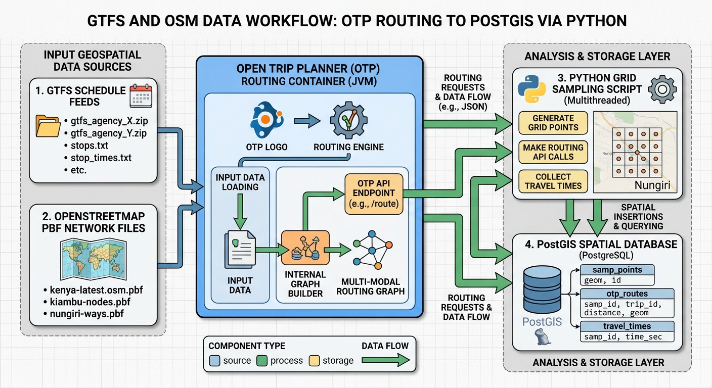
1. Architecture and data flow for Multi-Modal Public Transit Isochrones
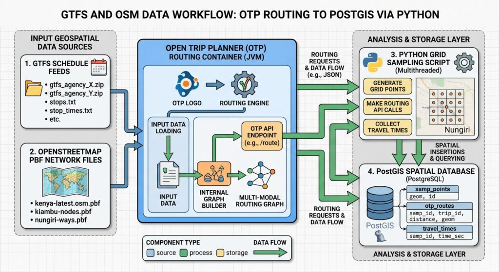
The workflow contains four components:
- Network inputs: GTFS supplies transit stops, routes, trips, schedules, and service calendars. OSM supplies routable streets, footways, cycleways, and other mapped connections.
- Routing engine: OTP builds a graph that connects the transit network to accessible streets and answers journey-planning requests through its GraphQL API.
- Python processing: Python creates a regular destination grid, queries OTP for travel durations, and associates the results with spatial cells.
- Spatial analysis: PostGIS stores the cell geometries, creates time-threshold polygons, and intersects them with population, healthcare, education, and employment datasets.
This separation keeps routing, orchestration, and spatial analysis independent. Record the graph version, GTFS feed dates, OSM snapshot, origin, departure time, permitted modes, and grid size for each run.
2. Assemble and validate the input data
Download GTFS Schedule ZIP files from the transport operators or relevant transport authority. Include all significant services in the study area, such as buses, commuter rail, metro, tram, and ferry where applicable.
Validate the feeds using the MobilityData GTFS Schedule Validator. Inspect stops.txt, routes.txt, trips.txt, stop_times.txt, calendar.txt, and calendar_dates.txt. In particular, verify that the selected analysis date has valid service and that stops are correctly located.
Obtain an OSM PBF extract covering the study area and a surrounding buffer. Clipping data too tightly can create artificial network endpoints and remove useful connections beyond the boundary.
Check pedestrian paths, crossings, station entrances, bridges, and cycling connections. Missing links can create misleading travel times even when the GTFS feed passes validation.
Keep the original datasets unchanged. Record their download dates and maintain a separate log of any feed corrections.
3. Configure OpenTripPlanner
Use a pinned OTP release and follow its official container documentation. Store the OSM extract, GTFS ZIP files, and configuration files in a mounted directory.
An example directory structure is:
transit-network/
├── region.osm.pbf
├── city-gtfs.zip
├── rail-gtfs.zip
├── build-config.json
├── router-config.json
└── graph.obj
The GTFS filenames should include gtfs, following OTP’s container workflow. Configure the transit service period to cover the dates being analyzed and use the correct timezone for the study area.
A typical container lifecycle is:
# Build and save the graph
docker run --rm \
  -e JAVA_TOOL_OPTIONS='-Xmx8g' \
  -v "$(pwd)/transit-network:/var/opentripplanner" \
  docker.io/opentripplanner/opentripplanner:<pinned-version> \
  --build --save

# Start the saved graph
docker run --rm -p 8080:8080 \
  -e JAVA_TOOL_OPTIONS='-Xmx8g' \
  -v "$(pwd)/transit-network:/var/opentripplanner" \
  docker.io/opentripplanner/opentripplanner:<pinned-version> \
  --load --serve
Replace <pinned-version> with an actual released tag. Allocate memory according to the graph’s size and inspect the build report for missing feeds, unlinked stops, and other import problems.
OTP 2 exposes a GraphQL API. Its usual GTFS endpoint is:
http://localhost:8080/otp/gtfs/v1The GraphiQL interface, when enabled, is generally available at http://localhost:8080/graphiql. Inspect the schema for the specific OTP release before implementing requests. Do not expose an unsecured development server to the public internet.
4. Generate the destination grid with Python
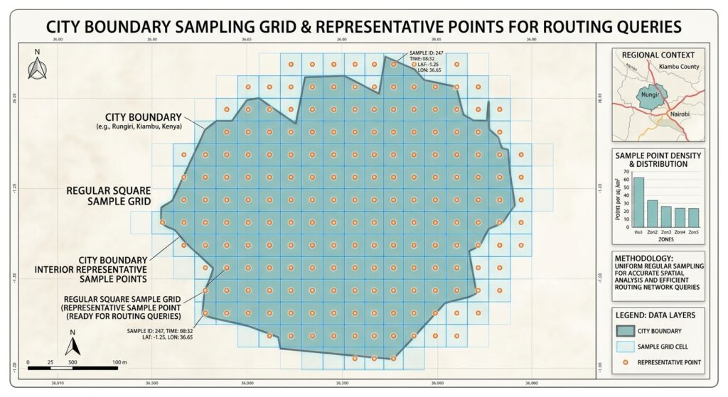
A destination grid converts a continuous study area into discrete locations where OTP can calculate travel times. Each cell receives a sample point, and Python submits that point to the router.
Grid resolution controls the trade-off between spatial detail and computation. A 500-metre grid typically requires fewer requests than a 100-metre grid, but produces a coarser accessibility boundary. Start with 250–500 metres for a city-scale analysis and refine the resolution only where necessary.
The following complete script:
- Reads a polygon or multipolygon study boundary from a GeoPackage, GeoJSON, Shapefile, or another supported vector format.
- Repairs invalid geometries and combines the polygon boundaries.
- Uses a projected coordinate reference system (CRS) with metre units.
- Creates a regular square grid and clips each cell to the study area.
- Generates a sample point inside every polygon component.
- Transforms cell geometries and sample points to WGS84 (EPSG:4326).
- Exports a GeoPackage for spatial processing and a CSV containing the sample coordinates for routing.
Install the dependencies
Create a Python environment and install GeoPandas, Shapely, and their dependencies:
python -m venv .venvActivate the environment on Windows:
.venv\Scripts\activateOr on Linux:
source .venv/bin/activateInstall the packages:
python -m pip install geopandas shapely pyproj pandasComplete script: generate_transit_grid.py
Save the following code as generate_transit_grid.py.
#!/usr/bin/env python3
"""
Generate a clipped destination grid for public-transit accessibility analysis.

Outputs:
    1. GeoPackage containing clipped polygon cells and sample coordinates.
    2. CSV containing cell IDs, sample longitude/latitude, and grid metadata.

Usage:
    python generate_transit_grid.py \
        --boundary data/study_area.gpkg \
        --cell-size 300 \
        --metric-crs auto \
        --gpkg-output output/transit_grid.gpkg \
        --csv-output output/transit_grid_samples.csv
"""

import argparse
import math
from pathlib import Path

import geopandas as gpd
import pandas as pd
from shapely import make_valid, union_all
from shapely.geometry import Point, box


WGS84 = "EPSG:4326"


def polygon_parts(geometry):
    """Return all Polygon components from a geometry."""
    if geometry is None or geometry.is_empty:
        return []

    if geometry.geom_type == "Polygon":
        return [geometry]

    if geometry.geom_type in ("MultiPolygon", "GeometryCollection"):
        parts = []
        for component in geometry.geoms:
            parts.extend(polygon_parts(component))
        return parts

    # Ignore lines and points returned by geometry repair.
    return []


def load_study_area(path, layer=None):
    """Read, repair, and dissolve polygon boundaries."""
    read_options = {}
    if layer:
        read_options["layer"] = layer

    boundaries = gpd.read_file(path, **read_options)

    if boundaries.empty:
        raise ValueError("The boundary dataset contains no features.")

    if boundaries.crs is None:
        raise ValueError(
            "Input CRS is missing. Define the correct source CRS "
            "before running this script."
        )

    geometries = []
    for geometry in boundaries.geometry:
        if geometry is None or geometry.is_empty:
            continue

        repaired = make_valid(geometry)
        geometries.extend(polygon_parts(repaired))

    if not geometries:
        raise ValueError(
            "No valid polygon geometry was found in the input dataset."
        )

    study_area = union_all(geometries)

    # Dissolve again after repair and retain polygonal components only.
    geometries = polygon_parts(study_area)
    if not geometries:
        raise ValueError("The dissolved boundary contains no polygons.")

    return boundaries, union_all(geometries)


def select_metric_crs(boundaries, requested_crs):
    """
    Select a projected CRS for metre-based grid construction.

    'auto' estimates an appropriate UTM CRS from the input bounds.
    For large or multi-zone areas, supply a suitable local projection.
    """
    if requested_crs.lower() != "auto":
        metric_crs = requested_crs
    else:
        metric_crs = boundaries.estimate_utm_crs()
        if metric_crs is None:
            raise ValueError(
                "Could not estimate a projected CRS. "
                "Supply --metric-crs with an appropriate projected CRS."
            )

    projected = gpd.GeoSeries([], crs=metric_crs)
    if not projected.crs.is_projected:
        raise ValueError(
            f"{metric_crs} is not a projected CRS. "
            "Choose a CRS suitable for metre-based grid construction."
        )

    # Confirm the CRS uses metres rather than feet.
    axis_info = projected.crs.axis_info
    if not axis_info or any(
        not math.isclose(axis.unit_conversion_factor, 1.0, abs_tol=1e-9)
        for axis in axis_info[:2]
    ):
        raise ValueError(
            f"{metric_crs} does not use metres as its horizontal units. "
            "Supply a projected CRS whose units are metres."
        )

    return projected.crs


def generate_grid(study_area, cell_size, metric_crs, max_candidates):
    """Generate clipped polygon cells and interior sample points."""
    min_x, min_y, max_x, max_y = study_area.bounds

    # Align the regular grid to integer multiples of cell_size.
    ix_min = math.floor(min_x / cell_size)
    iy_min = math.floor(min_y / cell_size)
    ix_max = math.ceil(max_x / cell_size)
    iy_max = math.ceil(max_y / cell_size)

    candidate_count = (ix_max - ix_min) * (iy_max - iy_min)

    if candidate_count > max_candidates:
        raise ValueError(
            f"The grid requires up to {candidate_count:,} candidate cells, "
            f"exceeding the limit of {max_candidates:,}. "
            "Increase --cell-size or --max-candidates."
        )

    cell_records = []
    sample_points = []
    cell_id = 1

    for grid_i in range(ix_min, ix_max):
        x_min = grid_i * cell_size
        x_max = x_min + cell_size

        for grid_j in range(iy_min, iy_max):
            y_min = grid_j * cell_size
            y_max = y_min + cell_size

            square = box(x_min, y_min, x_max, y_max)

            if not square.intersects(study_area):
                continue

            clipped = square.intersection(study_area)

            # One row per polygon component avoids assigning one sample
            # time to multiple disconnected pieces within the same square.
            for part_number, polygon in enumerate(
                polygon_parts(clipped), start=1
            ):
                if polygon.is_empty or polygon.area <= 0:
                    continue

                # Guaranteed to lie inside the clipped polygon.
                sample_point = polygon.representative_point()

                cell_records.append({
                    "cell_id": cell_id,
                    "grid_i": grid_i,
                    "grid_j": grid_j,
                    "part_no": part_number,
                    "cell_size_m": float(cell_size),
                    "cell_area_m2": float(polygon.area),
                    "metric_crs": str(metric_crs),
                    "geometry": polygon,
                })

                sample_points.append(sample_point)
                cell_id += 1

    if not cell_records:
        raise ValueError(
            "No grid cells were generated. Check the boundary and CRS."
        )

    cells_metric = gpd.GeoDataFrame(
        cell_records,
        geometry="geometry",
        crs=metric_crs,
    )

    points_metric = gpd.GeoDataFrame(
        {"cell_id": cells_metric["cell_id"].to_numpy()},
        geometry=sample_points,
        crs=metric_crs,
    )

    return cells_metric, points_metric


def main():
    parser = argparse.ArgumentParser(
        description="Generate a study-area-clipped transit destination grid."
    )
    parser.add_argument(
        "--boundary",
        required=True,
        help="Input polygon boundary file.",
    )
    parser.add_argument(
        "--layer",
        default=None,
        help="Optional input layer name, for example a GeoPackage layer.",
    )
    parser.add_argument(
        "--cell-size",
        type=float,
        default=300.0,
        help="Grid cell width in metres. Default: 300.",
    )
    parser.add_argument(
        "--metric-crs",
        default="auto",
        help="Projected metre-based CRS, such as EPSG:32737, or 'auto'.",
    )
    parser.add_argument(
        "--gpkg-output",
        default="output/transit_grid.gpkg",
        help="Output GeoPackage path.",
    )
    parser.add_argument(
        "--csv-output",
        default="output/transit_grid_samples.csv",
        help="Output CSV path.",
    )
    parser.add_argument(
        "--max-candidates",
        type=int,
        default=250000,
        help="Maximum candidate squares allowed. Default: 250000.",
    )
    args = parser.parse_args()

    if args.cell_size <= 0:
        parser.error("--cell-size must be greater than zero.")

    if args.max_candidates <= 0:
        parser.error("--max-candidates must be greater than zero.")

    boundary_path = Path(args.boundary)
    if not boundary_path.exists():
        parser.error(f"Boundary file does not exist: {boundary_path}")

    boundaries, study_area = load_study_area(
        boundary_path, layer=args.layer
    )

    metric_crs = select_metric_crs(boundaries, args.metric_crs)
    study_area_metric = gpd.GeoSeries(
        [study_area], crs=boundaries.crs
    ).to_crs(metric_crs).iloc[0]

    cells_metric, points_metric = generate_grid(
        study_area=study_area_metric,
        cell_size=args.cell_size,
        metric_crs=metric_crs,
        max_candidates=args.max_candidates,
    )

    # Convert both polygons and sample locations to longitude/latitude.
    cells_wgs84 = cells_metric.to_crs(WGS84)
    points_wgs84 = points_metric.to_crs(WGS84)

    cells_wgs84["sample_lon"] = points_wgs84.geometry.x.to_numpy()
    cells_wgs84["sample_lat"] = points_wgs84.geometry.y.to_numpy()

    gpkg_path = Path(args.gpkg_output)
    csv_path = Path(args.csv_output)

    gpkg_path.parent.mkdir(parents=True, exist_ok=True)
    csv_path.parent.mkdir(parents=True, exist_ok=True)

    cells_wgs84.to_file(
        gpkg_path,
        layer="transit_grid",
        driver="GPKG",
        index=False,
    )

    # CSV preserves the cell IDs used to join results back to polygons.
    cells_wgs84.drop(columns="geometry").to_csv(
        csv_path,
        index=False,
    )

    print(f"Metric CRS: {metric_crs}")
    print(f"Cell size: {args.cell_size:g} metres")
    print(f"Generated cells: {len(cells_wgs84):,}")
    print(f"GeoPackage: {gpkg_path.resolve()}")
    print(f"Sample CSV: {csv_path.resolve()}")
    print("Sample coordinates are EPSG:4326 longitude/latitude.")


if __name__ == "__main__":
    main()
Run the grid generator
For example, use a 300-metre grid for a study area stored in a GeoPackage:
python generate_transit_grid.py \
  --boundary data/study_area.gpkg \
  --layer study_area \
  --cell-size 300 \
  --metric-crs auto \
  --gpkg-output output/transit_grid.gpkg \
  --csv-output output/transit_grid_samples.csv
For a study area in Nairobi, an appropriate local projected CRS may be selected explicitly, for example EPSG:32737, if it suits the dataset’s extent and accuracy requirements:
python generate_transit_grid.py \
  --boundary data/nairobi_boundary.gpkg \
  --cell-size 300 \
  --metric-crs EPSG:32737
The auto option estimates a UTM CRS from the source boundary. For large study areas spanning multiple UTM zones, select a projection suitable for the full region rather than relying on automatic selection.
The script produces:
transit_grid.gpkg: clipped polygon cells, unique IDs, cell areas, and sample coordinates.transit_grid_samples.csv: one row per cell with the same ID, longitude, latitude, and grid metadata.
Each clipped polygon component gets its own ID and its own representative sample point. This avoids assigning one travel-time observation to multiple disconnected polygon pieces within a single grid square.
The CSV coordinates are in longitude, latitude order. Use the sample latitude and longitude for OTP requests, and retain cell_id to join routing results back to the matching polygons.
5. Query OTP with Python
Once the grid exists, Python can iterate over the sample CSV, query OTP, and persist the travel time for each sample.
Use a fixed departure timestamp with the correct local timezone. Define the mode policy explicitly: for example, walking plus transit, or cycling access plus transit where the graph and routing configuration support it. Do not assume every combination of bicycle, walking, and public transport is valid in OTP.
A minimal request pattern using OTP’s GraphQL API is illustrated below. Confirm the input types and fields against your installed OTP version’s GraphiQL schema.
import requests

OTP_URL = "http://localhost:8080/otp/gtfs/v1"

QUERY = """
query {
  __typename
}
"""

def check_otp():
    response = requests.post(
        OTP_URL,
        json={"query": QUERY},
        timeout=30,
    )
    response.raise_for_status()

    payload = response.json()
    if payload.get("errors"):
        raise RuntimeError(payload["errors"])

    return payload["data"]
This initial request checks API availability; it does not calculate a journey. Replace the query with the planConnection operation and supported origin, destination, departure-time, and mode inputs from the installed OTP schema. Extract the relevant itinerary duration and convert it to seconds. Store failed or route-less requests as NULL, together with the routing errors, rather than treating missing routes as zero-minute journeys.
The travel-time query loop should perform these operations for each CSV row:
- Read
cell_id,sample_lon, andsample_lat. - Submit a destination query from the chosen origin to the sample point.
- Record the best valid itinerary duration under the specified mode and departure-time rules.
- Save the result against
cell_id, then checkpoint progress.
Begin with a small test set before running the complete grid. Add conservative concurrency, retries for temporary HTTP failures, request logging, and checkpoints so that a large study can resume after an interruption.
Important analytical limitation: OTP itinerary queries are not equivalent to exhaustive network analysis. Querying a sample of destinations can approximate a travel-time surface, but the result depends on the grid, the routing request, service calendars, and itinerary-selection behavior. For large regional analysis requiring more systematic travel-time surfaces, evaluate purpose-built tools such as R5.
6. Store and analyze the samples in PostGIS
Create a table to store sampled travel times and clipped cell geometries:
CREATE TABLE transit_samples (
    run_id           text NOT NULL,
    cell_id          bigint NOT NULL,
    origin_id        text NOT NULL,
    departure_time   timestamptz NOT NULL,
    travel_seconds   integer,
    cell_geom        geometry(Polygon, 4326) NOT NULL,
    PRIMARY KEY (run_id, origin_id, departure_time, cell_id),
    CHECK (travel_seconds IS NULL OR travel_seconds >= 0)
);

CREATE INDEX transit_samples_geom_gix
    ON transit_samples USING GIST (cell_geom);
Load the generated GeoPackage into a staging table, then join routing results by cell_id and insert them into transit_samples. If using ogr2ogr to import the grid, retain the polygon geometry and sample-coordinate attributes. Keep the routing results in a separate table until they have been matched and validated.
Next, dissolve cells that meet each travel-time threshold:
CREATE TABLE transit_isochrones (
    run_id          text NOT NULL,
    origin_id       text NOT NULL,
    departure_time  timestamptz NOT NULL,
    cutoff_seconds  integer NOT NULL,
    geom            geometry(MultiPolygon, 4326) NOT NULL,
    PRIMARY KEY (run_id, origin_id, departure_time, cutoff_seconds)
);

CREATE INDEX transit_isochrones_geom_gix
    ON transit_isochrones USING GIST (geom);
Generate the catchments:
INSERT INTO transit_isochrones
    (run_id, origin_id, departure_time, cutoff_seconds, geom)
SELECT
    s.run_id,
    s.origin_id,
    s.departure_time,
    c.cutoff_seconds,
    ST_Multi(
        ST_CollectionExtract(ST_Union(s.cell_geom), 3)
    )::geometry(MultiPolygon, 4326)
FROM transit_samples AS s
CROSS JOIN (VALUES (900), (1800), (2700)) AS c(cutoff_seconds)
WHERE s.travel_seconds IS NOT NULL
  AND s.travel_seconds <= c.cutoff_seconds
GROUP BY
    s.run_id,
    s.origin_id,
    s.departure_time,
    c.cutoff_seconds;
The three cutoffs represent 15, 30, and 45 minutes. ST_Union dissolves boundaries between neighboring reachable cells, while ST_CollectionExtract retains polygonal components.
Because each input cell is clipped to the study area, the final catchment is also constrained by that boundary. Document this when interpreting results near the edge of the modeled region.
Check geometry validity and area:
SELECT
    origin_id,
    cutoff_seconds,
    ST_IsValid(geom) AS valid_geometry,
    ST_Area(geom::geography) / 1000000.0 AS area_km2
FROM transit_isochrones;
Spatial indexes are important when testing catchments against large opportunity datasets. PostGIS documents how index-aware predicates can accelerate spatial filtering in its spatial index FAQ.
For example, count clinics intersecting the 30-minute catchment:
SELECT COUNT(*) AS clinics_reachable
FROM clinics AS c
JOIN transit_isochrones AS i
  ON ST_Intersects(i.geom, c.geom)
WHERE i.run_id = 'weekday-am-walk-transit'
  AND i.origin_id = 'central_station'
  AND i.cutoff_seconds = 1800;
For population coverage, overlay the catchment with census grids or administrative boundaries. Counting a whole district because any part intersects can overstate coverage. Where appropriate, use area-weighted population allocation or a finer population grid, documenting any assumption that population is uniformly distributed within source polygons.
7. Validate the catchments
Validate the workflow before interpreting its results.
Routing checks: Compare selected sample travel times with manually inspected OTP itineraries. Test walk-only, bus, rail, and transfer journeys wherever these modes exist.
Network checks: Inspect unreachable sample points, disconnected areas, and cells associated with missing services. Confirm that these reflect genuine network limitations rather than invalid feeds or missing OSM links.
Spatial checks: Ensure catchments expand with increasing time thresholds under consistent assumptions. Check polygon validity, unexpected holes, isolated fragments, and the effect of grid resolution.
Departure time is part of the model. Repeat the analysis for representative weekday peak, weekday off-peak, and weekend departures when the objective is to compare accessibility patterns. A single 08:00 output should be described as accessibility for that departure time and date, not as a universal measure of transit access.
Finally, distinguish reachability from accessibility. An isochrone estimates where travel may be possible within a given time; it does not directly measure how many jobs, clinics, schools, or residents are reachable. Combine the polygons with appropriate opportunity datasets to answer those questions.
Image placeholder

The map legend should explain the travel-time thresholds, departure date and time, permitted modes, and grid resolution.
SEO best practices and internal linking
Use the primary keyword naturally in the title, introduction, and a relevant heading. Support it with variations such as “public transport catchment areas,” “transit accessibility mapping,” and “schedule-aware travel-time surfaces” rather than repeating the same phrase unnaturally.
Add contextual internal links to related guides:
Replace the example paths with the actual published URLs. The first link provides a broader GTFS accessibility workflow; the second shows how catchments can support healthcare-equity analysis.
Summary
Building multi-modal public transit isochrones requires more than drawing buffers around stops. GTFS schedules and OSM network data feed OTP, Python generates a spatial sampling grid and retrieves journey durations, and PostGIS stores the results and constructs approximate catchment polygons.
The grid-generation script provides the missing spatial foundation: a reproducible grid in a metre-based CRS, clipped polygons, unique cell IDs, and sample coordinates suitable for OTP requests. The accuracy of the final catchments still depends on network completeness, departure-time assumptions, routing configuration, and grid resolution.
With explicit assumptions, validated inputs, indexed spatial tables, and traceable outputs, this workflow provides a practical starting point for assessing access to jobs, schools, healthcare, and other essential urban services.
Technical references: OTP API overview, OTP container documentation, GTFS validation, GeoPandas vector I/O, Shapely geometry operations, and PostGIS spatial indexes.