
Introduction: Scaling PostGIS Beyond a Single Large Table

Effective management of enterprise geospatial workflows requires comprehensive PostGIS Table Partitioning Spatial Index Tuning to maintain high query performance. Enterprise geospatial systems increasingly process billions of GPS observations, satellite-derived features, road-network segments, environmental measurements, and administrative boundaries. At this scale, a spatial query that once returned results in milliseconds may begin taking seconds or minutes, even when a GiST spatial index exists.
The difficulty is not simply the number of records. Performance depends on how efficiently PostgreSQL narrows the candidate rows, how much of the spatial index and table must be accessed, whether frequently accessed data fits in memory, and how effectively the query planner estimates the workload.
For example, a query searching GPS observations inside a small geographic area over the last 24 hours should not need to examine several years of historical observations. If the database cannot eliminate irrelevant data early, it may spend substantial time traversing indexes, reading table pages, and evaluating spatial predicates.
PostGIS table partitioning and spatial index tuning solve related but different problems. A GiST index accelerates spatial candidate selection within a table or partition. Partitioning divides a large logical table into smaller physical relations, allowing PostgreSQL to exclude entire partitions when a query constrains the partition key. PostgreSQL also supports fast archival operations by detaching or dropping obsolete partitions. These advantages depend on the workload and partition design; partitioning alone does not guarantee faster queries.
When should you partition a PostGIS table?
Partitioning becomes worth evaluating when the table’s working set and indexes are difficult to manage, query latency degrades despite appropriate indexing, or retention and bulk-loading operations are expensive. PostgreSQL’s documentation identifies table size relative to available memory as one useful rule of thumb, but there is no universal row-count threshold. Benchmark the actual workload rather than adopting a fixed rule.
Three strategies deserve consideration:
| Strategy | Best suited for | Main limitation |
|---|---|---|
| Range partitioning | GPS tracks, sensor readings, time-stamped features and historical records | Queries need usable time-range predicates for pruning |
| List partitioning | Explicit geographic regions, countries, administrative areas or tenants | Too many regions can create excessive partitions |
| Hash partitioning | Distributing rows across a fixed number of partitions by a key | Hash partitions do not inherently represent adjacent geographic areas |
A critical distinction: PostgreSQL does not automatically partition a table by the geometric footprint of each feature. Geography-based partitioning requires an explicit region or spatial-cell key, and spatial queries must constrain that key—or otherwise apply an appropriate pruning condition—to benefit from geographic partition elimination.
For many billion-row telemetry systems, monthly or daily range partitions on a timestamp provide the most straightforward starting point. Geographic partitioning can complement temporal partitioning when region-aware queries justify the additional complexity.
1. Design a PostGIS Table Partitioning Spatial Index Tuning Strategy
Before changing the schema, establish which columns appear most frequently in WHERE clauses, joins, and data-retention jobs.
An effective design often follows this sequence:
-
Use a timestamp range when time is the dominant filter and old data has a predictable lifecycle.
-
Use a region key when queries routinely operate on known geographic regions.
-
Consider hash partitioning when the principal objective is distributing records across partitions rather than isolating geographic neighborhoods.
-
Introduce subpartitioning only when measured performance or operational requirements justify another level of complexity.
Avoid creating hundreds or thousands of tiny partitions without evidence that they help. Excessive partition counts increase planning overhead, catalog complexity, index-management work, and maintenance coordination. Partitioning is also not a substitute for good query design, suitable hardware, or correct spatial indexing.
2. Set Up Declarative Table Partitioning in PostgreSQL
PostgreSQL’s declarative partitioning routes inserts through a parent table into child partitions according to a defined partition key. Applications can query the parent as though it were a single table while PostgreSQL determines which partitions to access.
The following example uses a large GPS observation table partitioned by observation time.
Step 1: Create the partitioned parent table
Ensure PostGIS is installed in the database before defining the geometry column.
CREATE EXTENSION IF NOT EXISTS postgis;

CREATE TABLE gps_events (
    event_id      bigint GENERATED BY DEFAULT AS IDENTITY,
    observed_at   timestamptz NOT NULL,
    region_id     integer NOT NULL,
    geom          geometry(Point, 4326) NOT NULL,
    attributes    jsonb
)
PARTITION BY RANGE (observed_at);
The important design choices are:
-
observed_atis the partition key, allowing PostgreSQL to eliminate partitions outside a requested time range. -
geomuses a consistent geometry type and SRID. -
region_idsupports region-specific filtering and can provide an additional attribute index. -
attributesstores optional, variable sensor metadata without introducing a large number of sparse columns.
For production systems, choose appropriate constraints and data types for the actual dataset. If globally unique identifiers or primary keys are required, account for PostgreSQL’s partitioned uniqueness rules: a PRIMARY KEY or UNIQUE constraint on the partitioned parent generally must include all partition-key columns. An identity column alone does not provide a global uniqueness guarantee.
Step 2: Create time-based partitions
Suppose the system receives continuous observations and most queries use monthly reporting periods.
CREATE TABLE gps_events_2026_10
PARTITION OF gps_events
FOR VALUES FROM ('2026-10-01 00:00:00+00')
             TO ('2026-11-01 00:00:00+00');

CREATE TABLE gps_events_2026_11
PARTITION OF gps_events
FOR VALUES FROM ('2026-11-01 00:00:00+00')
             TO ('2026-12-01 00:00:00+00');
These examples deliberately use explicit UTC boundaries. PostgreSQL range partitions include the lower bound and exclude the upper bound, so observations exactly at midnight on November 1 belong to the November partition rather than the October partition.
Choose partition intervals according to ingestion rates, query windows, retention requirements, and index size. Monthly partitions may work for historical environmental observations; daily or weekly partitions may be more suitable for very high-volume telemetry. The smallest possible partition is not necessarily the best one.
A production system should automate partition creation ahead of incoming data. Without a matching partition, an insert fails unless a suitable default partition exists. A default partition can provide a safety net, but it needs monitoring and careful handling when new partitions are attached.
Step 3: Apply the appropriate partitioning model
When the workload demands geographic separation, a list-partitioned table can use a stable region identifier:
CREATE TABLE regional_events (
    event_id    bigint GENERATED BY DEFAULT AS IDENTITY,
    region_id   text NOT NULL,
    observed_at timestamptz NOT NULL,
    geom        geometry(Point, 4326) NOT NULL
)
PARTITION BY LIST (region_id);

CREATE TABLE regional_events_north
PARTITION OF regional_events
FOR VALUES IN ('north');

CREATE TABLE regional_events_south
PARTITION OF regional_events
FOR VALUES IN ('south');
A query containing WHERE region_id = 'north' can eliminate unrelated region partitions. However, a query that only tests ST_Intersects(geom, ...) does not automatically tell PostgreSQL which region partition contains the matching features. Your application or spatial-query layer must identify the relevant regions and include suitable region predicates where feasible.
For spatial-grid workloads, assign each observation a stable cell identifier during ingestion. A hash-partitioned design can distribute those identifiers across a fixed number of child tables:
CREATE TABLE grid_events (
    event_id bigint GENERATED BY DEFAULT AS IDENTITY,
    cell_id  bigint NOT NULL,
    geom     geometry(Point, 4326) NOT NULL
)
PARTITION BY HASH (cell_id);

CREATE TABLE grid_events_p0
PARTITION OF grid_events
FOR VALUES WITH (MODULUS 4, REMAINDER 0);

CREATE TABLE grid_events_p1
PARTITION OF grid_events
FOR VALUES WITH (MODULUS 4, REMAINDER 1);

CREATE TABLE grid_events_p2
PARTITION OF grid_events
FOR VALUES WITH (MODULUS 4, REMAINDER 2);

CREATE TABLE grid_events_p3
PARTITION OF grid_events
FOR VALUES WITH (MODULUS 4, REMAINDER 3);
Important: These hash partitions distribute cell identifiers by hash remainder; they do not group neighboring cells together. A query filtered only by geometry will generally need to consider all hash partitions. Use a region-list design when geographic locality is the main objective, and hash partitioning when balanced distribution is more important.
For workloads needing both temporal and regional pruning, PostgreSQL supports subpartitioning. For example, a time-partitioned parent can have monthly children that are themselves partitioned by region. Test this carefully: every additional partitioning level creates operational and planning overhead.
3. Create and Tune GiST Spatial Indexes
Partitioning reduces the number of tables PostgreSQL must search when pruning is possible. It does not replace spatial indexes on the surviving data.
PostGIS commonly uses a GiST index, which implements an R-tree-style spatial indexing strategy for geometry. A spatial index stores bounding-box information rather than performing every exact geometric comparison during index traversal. Candidate matches are subsequently checked using the required spatial predicate.
Step 4: Build indexes on the parent table
For a new partitioned table, create indexes on the parent:
CREATE INDEX gps_events_geom_gix
ON gps_events
USING GIST (geom);

CREATE INDEX gps_events_observed_at_bix
ON gps_events (observed_at);

CREATE INDEX gps_events_region_bix
ON gps_events (region_id);
The GiST index accelerates spatial filtering. The B-tree indexes serve conventional timestamp and region comparisons, although PostgreSQL may choose a different plan depending on selectivity and available statistics.
Creating an index on a partitioned parent establishes a partitioned index and corresponding indexes on its child partitions. Newly created partitions can also receive matching indexes through the parent index definition.
After creation, check that the child indexes exist and are valid. Use pg_indexes to inspect index definitions:
SELECT schemaname, tablename, indexname, indexdef
FROM pg_indexes
WHERE tablename LIKE 'gps_events%'
ORDER BY tablename, indexname;
Step 5: Index large existing tables with minimal disruption
For an existing production hierarchy, index creation can be a significant operational event. PostgreSQL does not support CREATE INDEX CONCURRENTLY directly on a partitioned parent. Instead, create matching indexes concurrently on the individual leaf partitions and attach them to an initially incomplete partitioned index.
For example:
-- Create an initially invalid parent index definition.
CREATE INDEX gps_events_geom_gix
ON ONLY gps_events
USING GIST (geom);

-- Build the actual index without blocking ordinary writes
-- to an existing leaf partition.
CREATE INDEX CONCURRENTLY
gps_events_2026_10_geom_gix
ON gps_events_2026_10
USING GIST (geom);

-- Attach the child index to the parent index.
ALTER INDEX gps_events_geom_gix
ATTACH PARTITION gps_events_2026_10_geom_gix;
Repeat the child-index creation and attachment for the remaining leaf partitions. The parent index becomes valid when all required partition indexes are attached. Run concurrent index builds outside an explicit transaction block, and monitor failures and invalid indexes. This approach reduces write disruption compared with building all indexes on a large hierarchy in one blocking operation, although index builds still consume disk I/O and CPU.
Step 6: Match indexes to query patterns
A spatial GiST index is not the answer to every query. Tune the complete access pattern:
-
Spatial searches: Use index-aware predicates such as
ST_IntersectsandST_DWithinwhere appropriate. -
Time filtering: Retain the range predicate on the partition key; use a B-tree index when it benefits the plan.
-
Attribute filtering: Index selective fields frequently used alongside spatial conditions.
-
Append-heavy time series: Evaluate BRIN indexes for naturally ordered or spatially correlated data when the smaller index size and lower maintenance cost justify the trade-off.
PostGIS documents GiST, BRIN, and SP-GiST as distinct spatial-index options. BRIN summarizes ranges of table blocks and is most effective when the physical row order correlates with the indexed values; it is not a universal replacement for GiST.
Don’t add every possible index. Each additional index increases storage requirements and the work needed for inserts, updates, and maintenance. Benchmark the actual spatial predicates and combinations of filters used by the application.
4. Verify Partition Pruning with EXPLAIN ANALYZE
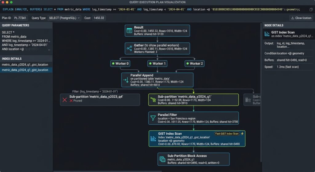
Partition pruning is the process by which PostgreSQL excludes partitions that cannot contain rows satisfying a query’s partition-key conditions. It is one of the most important benefits of declarative partitioning, but it only works when the query and partition design provide the necessary information.
Step 7: Run a spatial query with temporal constraints
The following query searches a geographic window over a limited reporting period:
EXPLAIN (ANALYZE, BUFFERS, VERBOSE, SETTINGS)
SELECT event_id, observed_at, geom
FROM gps_events
WHERE observed_at >= '2026-10-01 00:00:00+00'
  AND observed_at <  '2026-11-01 00:00:00+00'
  AND ST_Intersects(
      geom,
      ST_MakeEnvelope(-1, 35, 1, 37, 4326)
  );
The timestamp predicates constrain the query to October’s partition. ST_Intersects includes a bounding-box comparison that can use an available spatial index before performing the exact geometry test.
Inspect the execution plan for:
| Plan indicator | What it tells you |
|---|---|
Append or Parallel Append |
PostgreSQL is combining results from child relations; these nodes alone do not prove effective pruning |
| Only the October child appears | Irrelevant partitions were excluded during planning |
Subplans Removed or subplans marked never executed |
Can indicate execution-time partition pruning |
Index Scan or Bitmap Index Scan using a GiST index |
The spatial index is participating in candidate selection |
Seq Scan on a child partition |
May be appropriate for a small partition or a query matching a large proportion of its rows |
| Large actual-versus-estimated row differences | May indicate stale statistics or a selectivity-estimation problem |
| Many shared buffer reads | The query is reading substantial data from storage rather than finding it all in cache |
PostgreSQL supports buffer reporting and execution-time measurements through EXPLAIN; these metrics help distinguish I/O pressure, inefficient access paths, and inaccurate estimates.
[Image 1: PostgreSQL query plan showing partition pruning versus sequential scan on billion-row table]
Alt text: “PostgreSQL explain analyze execution plan output showing efficient partition pruning versus unindexed sequential table scans on billion-row spatial datasets.”
Editorial guidance: Use a genuine EXPLAIN (ANALYZE, BUFFERS) output from a representative dataset. Annotate the selected child partitions, the GiST scan, actual row counts, buffer activity, and execution time. Avoid presenting illustrative timings as measured production results.
Step 8: Compare the partitioned and unpartitioned plans
Use the same representative filters, geometry, and result columns when comparing designs. On a test environment, run the equivalent query against a baseline unpartitioned table with appropriate indexes.
Evaluate:
-
How many partitions were scanned?
-
How many rows and index entries were examined?
-
How many buffers were read and hit?
-
How accurately did estimated row counts match actual counts?
-
Did execution time improve across repeated tests under realistic cache and concurrency conditions?
For a controlled experiment, inspect the setting:
SHOW enable_partition_pruning;Normally, partition pruning should be enabled. Do not disable it as a routine optimization strategy.
Avoid assuming that forcing an index scan must always improve performance. A broad query retrieving a large share of the rows may run faster with a sequential scan. The objective is to minimize total workload cost, not to eliminate every sequential scan.
Also test parameterized queries with realistic values. Depending on the plan and parameter values, partition elimination may occur at planning time or execution time. A query can therefore show a more complicated plan than expected while still avoiding execution of irrelevant partitions.
5. Maintenance and Bloat Management
Billion-row database performance is an ongoing operational concern. Updates and deletes leave obsolete tuple versions that PostgreSQL must reclaim through vacuuming, while statistics updates help the planner estimate query costs. PostGIS index maintenance and partition lifecycle management must be included in this routine.
Step 9: Maintain table statistics and vacuum regularly
Use targeted maintenance for heavily loaded or frequently changed partitions:
VACUUM (ANALYZE) gps_events_2026_10;
VACUUM (ANALYZE) gps_events_2026_11;
These commands reclaim space for reuse and refresh statistics for the selected leaf partitions. Also run ANALYZE gps_events; on the partitioned parent when needed so the planner has up-to-date information at the parent level, particularly after substantial data changes. Partitioned parent tables require attention because their overall statistics are not automatically refreshed merely by vacuuming the children.
For a mostly append-only partition, focus on insert-driven statistics updates and freezing requirements. For an update-heavy partition, monitor dead tuples, autovacuum activity, and index growth. For a partition that has become immutable, ensure its statistics remain representative after bulk loading.
Step 10: Tune autovacuum per partition
PostgreSQL provides table-level storage parameters for adjusting autovacuum behavior. This is useful when the default scale factors are too slow to trigger maintenance on a very large table. The following settings are illustrative starting points, not universal production values.
ALTER TABLE gps_events_2026_10 SET (
    autovacuum_vacuum_scale_factor = 0.02,
    autovacuum_analyze_scale_factor = 0.01,
    autovacuum_vacuum_threshold = 50000,
    autovacuum_analyze_threshold = 50000
);
With a 2% vacuum scale factor, the scale-factor component of the trigger rises with table size, while the threshold adds a baseline count. These values should be chosen based on update rates, insert volume, dead-tuple growth, maintenance capacity, and observed statistics freshness.
Monitor at least the following:
-
pg_stat_user_tablesfor sequential scans, index scans, tuple changes, and vacuum/analyze timestamps. -
pg_stat_progress_vacuumfor vacuum operations currently in progress. -
Disk utilization and index sizes, including changes across individual partitions.
-
Autovacuum logs and transaction ID age to identify delayed maintenance or freeze pressure.
Don’t simply disable autovacuum to reduce background activity. Delayed vacuuming may allow dead tuples and index bloat to accumulate and can create transaction ID wraparound risk. PostgreSQL’s vacuuming documentation explains why routine vacuuming is required and why VACUUM FULL is not a routine substitute: it rewrites the table and requires an exclusive lock.
Step 11: Control bloat and manage partition lifecycles
For time-partitioned datasets, use partition operations instead of massive row-by-row deletions when the retention policy aligns with partition boundaries. Dropping or detaching an obsolete partition can remove a large volume of data without the vacuum overhead associated with deleting those rows individually.
For example:
-- Detach a historical partition before archival or disposal.
ALTER TABLE gps_events
DETACH PARTITION gps_events_2024_01;
Choose the detach approach supported by your PostgreSQL version and operational requirements. Validate dependencies, downstream consumers, backups, and retention policies before removing data. If the detached relation is retained for archival, ensure it is no longer written through the parent.
When an index grows disproportionately, first investigate dead tuples, update churn, query patterns, and maintenance history. REINDEX may be appropriate for a confirmed index-bloat issue, but it consumes resources and requires operational planning. Concurrent reindexing can reduce blocking in supported cases, though it is not free of resource costs. Avoid using table rewrites as a default maintenance habit.
6. Advanced Optimization Strategies for Enterprise Deployments
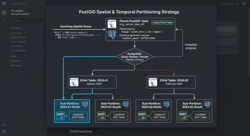
Partitioning and GiST indexes establish the foundation, but high-volume geospatial workloads often need additional tuning.
Step 12: Evaluate combined indexes and partition-wise operations
A spatial query may filter on region, time, and geometry simultaneously. PostgreSQL can sometimes combine separate indexes through bitmap operations, but a multicolumn index is not automatically faster.
For example, a conventional B-tree on region_id and a GiST index on geom may perform well when the planner can combine both filters. Test realistic data distributions before adding more indexes, particularly when the spatial predicate already eliminates most rows.
Partition-wise joins can also reduce work when compatible partitioned tables are joined on their partitioning keys. However, they introduce planning and execution trade-offs and should be benchmarked against ordinary joins. Avoid assuming they will help every spatial join.
Step 13: Consider parallel query execution
For queries scanning large portions of a partitioned dataset, parallel scans and parallel append operations may reduce elapsed time when CPU and storage bandwidth are available.
Test parallel execution under realistic concurrency. Increasing parallel workers can help a single analytical query but may reduce overall throughput when several large queries compete for the same CPUs or I/O resources.
For historical time-series tables, a BRIN index on a timestamp may complement GiST indexing when rows are physically correlated with time. For spatially ordered data, a spatial BRIN index may also be useful. Confirm the behavior with the specific PostGIS and PostgreSQL versions deployed.
Step 14: Design the partition architecture for operations
Client / Application
Spatial SQL with time, region and geometry predicates
Partitioned PostGIS parent table
Query planning · Partition pruning · Row routing
Time partitions
Range
Region partitions
List
Hash partitions
Key distribution
Child tables and local indexes
GiST geometry indexes · B-tree attribute indexes · Optional BRIN indexes
[Image 2: Architecture diagram of parent table routing spatial queries to child partitions]
Alt text: “System architecture diagram illustrating a parent PostGIS table routing incoming spatial queries to time-based and geography-based child partition tables.”
Editorial guidance: The diagram should distinguish logical routing from physical data access. Partitioning routes rows by the configured key, whereas the query planner determines which partitions to scan. Spatial indexes then narrow candidate features inside the selected child tables.
7. SEO Best Practices and Technical Interlinking
Strengthen this guide’s topical authority by connecting it to related database-engineering tutorials.
| Suggested internal article | Recommended anchor text |
|---|---|
/spatial-indexing-r-tree-b-tree-postgis/ |
Spatial indexing with R-trees and B-trees |
/postgis-raster-processing-optimization/ |
PostGIS raster processing and optimization |
/postgis-spatial-window-functions/ |
Spatial window functions in PostGIS |
These are suggested URL slugs, not verified existing pages; replace them with the corresponding published URLs on your website.
For the authoritative external reference, link to the official PostgreSQL documentation on table partitioning. It covers partition strategies, pruning, index behavior, and operational considerations.
Use the primary keyword naturally in the H1, introduction, one relevant subheading, and conclusion. Incorporate the secondary keywords in sections where they accurately describe the technical content. Include the two architecture and execution-plan illustrations with their supplied alt text, and ensure SQL examples are readable and copyable in the published article.
8. Summary and Enterprise Takeaways
Scaling multi-billion-row PostGIS tables requires a coordinated strategy rather than a single indexing trick.
First, partition around how the data is queried and retained. Temporal range partitioning is a strong baseline for time-series observations, while geographic list partitioning is useful when region-based filters are common. Hash partitioning distributes key values but does not inherently create geographic locality.
Second, tune GiST indexes within the partitioning architecture. Create spatial indexes on the parent or manage child indexes deliberately during production migrations. Maintain complementary B-tree indexes where they serve real query patterns, and evaluate BRIN indexes for physically correlated data.
Third, verify actual execution plans. Use EXPLAIN (ANALYZE, BUFFERS) to assess partition pruning, index usage, row estimates, and I/O. Remember that a sequential scan can be the optimal plan for small partitions or queries returning many rows.
Finally, make maintenance part of the architecture. Automate future partition creation, maintain statistics, tune autovacuum using measured workload behavior, monitor index growth, and implement partition-based retention where appropriate.
The central principle of PostGIS table partitioning and spatial index tuning is to minimize irrelevant work: eliminate unnecessary partitions first, identify spatial candidates efficiently within the remaining data, and validate that the resulting plan improves real production workloads.
Enterprise scalability comes from matching physical storage design, query patterns, index maintenance, and workload monitoring—not simply from increasing the number of partitions or adding more indexes.