
Multimodal Accessibility Modeling with GTFS Data in GIS
1. Multimodal Accessibility Modeling GTFS GIS: Understanding GTFS Data
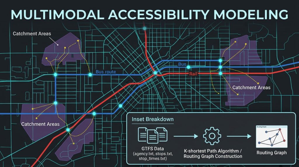
Conventional road network analysis answers questions such as how quickly a driver can travel between two locations, which roads provide the shortest route, or what area lies within a 15-minute drive. However, these methods do not adequately represent the travel experience of people who depend on public transportation, walking, or cycling.
A road-only routing model cannot reliably determine whether a bus is operating at a particular time, how long a passenger must wait, whether a connecting service is available, or how a missed transfer affects total journey time. Even a short road distance between two neighborhoods can translate into a long public transport journey if the available services require indirect routes or infrequent transfers.
Multimodal accessibility modeling with GTFS and GIS addresses these limitations by combining street networks, public transit schedules, walking connections, and destination locations within a time-dependent transportation model.
The General Transit Feed Specification (GTFS) describes public transport services using standardized files containing stops, routes, trips, scheduled arrival and departure times, and service calendars. Routing engines can combine GTFS schedules with OpenStreetMap (OSM) street networks to calculate journeys that include walking to a stop, waiting for a vehicle, riding transit, transferring between services, and walking to the destination.
The official GTFS Schedule Reference defines the structure of these files and their relationships. OpenTripPlanner is an open-source routing engine designed to combine scheduled public transportation with walking, cycling, and other mobility modes. See the OpenTripPlanner documentation.
This guide develops a practical workflow for transportation planners who want to map public transport catchment areas and measure access to employment, healthcare, education, and other urban opportunities.
2. Understanding GTFS data
GTFS Schedule is usually distributed as a ZIP archive containing text files. These files describe the transit system’s network structure and the dates and times when services operate.
The primary files are:
| GTFS file | Function in accessibility modeling |
|---|---|
agency.txt |
Identifies transit agencies and defines the relevant time zone. |
stops.txt |
Stores stop and station identifiers, coordinates, and station relationships. |
routes.txt |
Defines public transport routes and their modes. |
trips.txt |
Identifies individual scheduled trips operating on particular services. |
stop_times.txt |
Stores scheduled arrivals and departures at stops along each trip. |
calendar.txt |
Defines regular weekly service and its start and end dates. |
calendar_dates.txt |
Adds or removes service on specific dates, including exceptions and holidays. |
shapes.txt |
Optionally describes the geographic paths followed by transit vehicles. |
transfers.txt |
Provides information about transfers between services. |
frequencies.txt |
Describes services operating at specified headways rather than only individual scheduled departure times. |
The main relationships connect routes to trips, trips to their scheduled stop times, and trips to service calendars. Stops provide the locations at which passengers access the transit network.
One important detail is that GTFS times can exceed 24:00:00. For example, 25:15:00 represents 1:15 AM on the following calendar day within the relevant service day. A preprocessing script should not automatically convert every GTFS time into an ordinary clock time without preserving its service-day meaning.
The official GTFS reference also defines optional station, pathway, accessibility, and other fields that can improve the realism of a transit model.
Why a transit schedule matters
Consider two neighborhoods located five kilometers apart.
A road-only model might estimate a short driving journey. A pedestrian network might show that the neighborhoods are also relatively close on foot. However, a public transport journey could require walking 800 meters to a stop, waiting 12 minutes, riding for 18 minutes, transferring to another service, and walking to the destination.
The result depends on more than geographic distance. It depends on the service operating on the selected date, the sequence of available departures, walking connections, and transfer opportunities.
For this reason, travel time transit network analysis must be timetable-aware when the objective is to estimate realistic public transport accessibility.
3. Step 1 — Source GTFS schedules and road network data
The first task is to obtain a transit feed and a street network covering the same geographic region.
3.1 Obtain GTFS data
Start with the official public transport agency or operator. Many agencies publish GTFS feeds on their websites or through open data portals.
If the operator does not provide a convenient download, consult the Transitland feed registry or other relevant regional transit-data catalogs.
Download the static GTFS ZIP archive and record its source, retrieval date, applicable service dates, and any known limitations.
For a regional model, ensure that the feed covers all relevant public transport operators. A feed containing only one bus company may omit rail, commuter buses, ferries, or other services needed to represent complete journeys.
3.2 Download OpenStreetMap data
GTFS describes public transport services but does not, by itself, provide a complete pedestrian network between every origin, stop, and destination.
OpenStreetMap supplies the street and pedestrian-network information needed for walking access, transfers, and destination access.
Obtain an appropriate regional extract from Geofabrik or another suitable OSM data provider. OpenTripPlanner commonly uses OSM in .osm.pbf format.
Download the network for the entire study region, including an adequate margin around the study boundary. A journey that begins inside the study area may use a transit route or transfer outside it.
Keep the GTFS feed and OSM extract from compatible geographic periods where practical. Check that important stops have nearby pedestrian-accessible street connections.
Remember to follow the OpenStreetMap attribution and licensing requirements.
3.3 Validate the GTFS feed before building a network
A structurally incomplete or outdated feed can produce misleading accessibility results. For example, a model may omit a service because its operating dates are incorrect, or fail to connect a stop because the pedestrian network does not reach its coordinates.
The following Python script performs basic checks on a local GTFS ZIP archive.
Install pandas if needed:
python -m pip install pandasSave the script as check_gtfs.py:
from pathlib import Path
from zipfile import ZipFile
import pandas as pd

GTFS_PATH = Path("agency.gtfs.zip")

# Core files used in an ordinary fixed-route GTFS feed.
REQUIRED_FILES = {
    "agency.txt",
    "stops.txt",
    "routes.txt",
    "trips.txt",
    "stop_times.txt",
}

# Read tables by filename, including archives that contain
# a subdirectory rather than placing files directly at the root.
def read_gtfs_table(archive, filename):
    matches = [
        name for name in archive.namelist()
        if Path(name).name == filename
    ]

    if not matches:
        return None

    with archive.open(matches[0]) as file:
        return pd.read_csv(file, dtype=str)


with ZipFile(GTFS_PATH) as archive:

    available = {
        Path(name).name
        for name in archive.namelist()
        if not name.endswith("/")
    }

    missing = REQUIRED_FILES - available

    if missing:
        raise ValueError(
            f"Required GTFS files are missing: {sorted(missing)}"
        )

    # Regular calendar definitions or explicit date exceptions
    # must be available according to the GTFS specification.
    if not (
        "calendar.txt" in available
        or "calendar_dates.txt" in available
    ):
        raise ValueError(
            "Neither calendar.txt nor calendar_dates.txt exists."
        )

    agency = read_gtfs_table(archive, "agency.txt")
    stops = read_gtfs_table(archive, "stops.txt")
    routes = read_gtfs_table(archive, "routes.txt")
    trips = read_gtfs_table(archive, "trips.txt")
    stop_times = read_gtfs_table(archive, "stop_times.txt")

    # Report basic table sizes.
    print("Agencies:", len(agency))
    print("Stops:", len(stops))
    print("Routes:", len(routes))
    print("Trips:", len(trips))
    print("Stop-time records:", len(stop_times))

    # Check important fields before attempting joins.
    required_columns = {
        "stops.txt": (stops, {"stop_id", "stop_lat", "stop_lon"}),
        "routes.txt": (routes, {"route_id"}),
        "trips.txt": (trips, {"trip_id", "route_id", "service_id"}),
        "stop_times.txt": (
            stop_times,
            {"trip_id", "stop_id", "stop_sequence"},
        ),
    }

    for filename, (table, columns) in required_columns.items():
        absent = columns - set(table.columns)

        if absent:
            raise ValueError(
                f"{filename} is missing columns: {sorted(absent)}"
            )

    # Verify that trip references resolve to valid records.
    if not trips["route_id"].isin(routes["route_id"]).all():
        raise ValueError("Some trips reference unknown route IDs.")

    if not stop_times["trip_id"].isin(trips["trip_id"]).all():
        raise ValueError("Some stop_times reference unknown trips.")

    if not stop_times["stop_id"].isin(stops["stop_id"]).all():
        raise ValueError("Some stop_times reference unknown stops.")

    # Confirm that stop coordinates can be interpreted numerically.
    lat = pd.to_numeric(stops["stop_lat"], errors="coerce")
    lon = pd.to_numeric(stops["stop_lon"], errors="coerce")

    invalid_coordinates = (
        lat.isna()
        | lon.isna()
        | ~lat.between(-90, 90)
        | ~lon.between(-180, 180)
    )

    print("Invalid stop coordinates:", int(invalid_coordinates.sum()))

    print("Basic GTFS integrity checks completed.")
Run the script:
python check_gtfs.pyThis is a basic integrity check, not a full GTFS compliance validator. It does not test every service-calendar relationship, stop-time sequence, transfer rule, or accessibility field.
Before proceeding, also verify that services are active on your intended analysis dates and that the feed covers the modes and operators needed for your study.
4. Step 2 — Build the multimodal routing network
You can perform GTFS-based accessibility analysis using QGIS with OpenTripPlanner, or use ArcGIS Pro with its public transit data model and Network Analyst extension.
The choice depends on available software, licensing, scale, and how much control you need over the routing engine.
Option A: QGIS and OpenTripPlanner
OpenTripPlanner combines OSM street networks with GTFS schedules to construct a multimodal routing graph.
A current QGIS plugin option is Easy-OTP, which automates temporal public transport accessibility analysis and offers workflows for isochrones, travel-time matrices, and accessibility surfaces. Its published implementation uses OpenTripPlanner 1.5.0, so verify the plugin’s requirements and compatibility before adopting it for a new deployment. See the Easy-OTP listing in the QGIS plugin repository.
The older OpenTripPlanner QGIS plugin also targets OTP 1.5. Do not assume that plugins written for OTP 1.5 will work with OTP 2.
For a new OTP 2 deployment, use the current OpenTripPlanner 2 documentation and connect through a compatible client or API integration.
Procedure
- Open QGIS and select Plugins → Manage and Install Plugins.
- Search for
Easy-OTPand install it if your QGIS version and project requirements are compatible. - Follow the plugin’s setup procedure for the routing engine and transit data. Confirm that both GTFS and OSM data cover the study area.
- Start or test the routing server using the plugin’s available tools.
- Load your neighborhood boundaries, population grid, job locations, healthcare facilities, and other relevant GIS layers.
- Use the plugin’s temporal accessibility or isochrone tools to calculate reachability for the selected departure-time scenarios.
- Export the resulting grids, isochrones, travel-time matrices, or accessibility indicators for further analysis in QGIS.
The plugin’s published functionality includes temporal accessibility surfaces, service-coverage calculations, isochrone generation, and origin-destination travel-time matrices. Consult its documentation for the configuration fields and output requirements associated with each tool.
Building a separate OpenTripPlanner 2 instance
For a standalone OTP 2 deployment, prepare a folder containing the routing engine, a GTFS feed, and an OSM extract.
Example directory:
otp_project/
├── otp-shaded-VERSION.jar
├── agency.gtfs.zip
├── region.osm.pbf
└── build-config.json
Here is an illustrative build-config.json:
{
  "transitServiceStart": "-P3M",
  "transitServiceEnd": "P1Y",
  "osm": [
    {
      "source": "region.osm.pbf"
    }
  ],
  "transitFeeds": [
    {
      "type": "gtfs",
      "source": "agency.gtfs.zip"
    }
  ]
}
The service range is an example; choose one appropriate to the feed’s actual service dates and the analysis period. See the OTP graph build configuration reference.
With a compatible OTP 2 JAR and Java runtime installed, build and save the routing graph using a command of this form:
java -Xmx4G -jar otp-shaded-VERSION.jar --build --save .Replace VERSION with the installed JAR version and execute the command from the directory containing the configuration and input data.
After the build succeeds, start the saved graph:
java -Xmx2G -jar otp-shaded-VERSION.jar --load .The memory limits are illustrative. Large regional graphs may need substantially more RAM. Check the build logs and resolve errors relating to GTFS dates, missing data, stop connectivity, or OSM coverage before generating accessibility maps.
The important distinction is that building a routing graph is not the same as generating an accessibility catchment. You must subsequently submit time-dependent routing or accessibility requests through a compatible interface.
Option B: ArcGIS Pro and Network Analyst
ArcGIS Pro provides tools for building a network dataset that includes scheduled public transportation.
The workflow uses the Network Analyst extension and a public transit data model that represents transit stops, lines, trips, and schedules. The official ArcGIS public transit analysis guide explains how the model supports time-dependent travel-time calculations.
Procedure
- Load GTFS source data and street centerlines or a suitable pedestrian network into your ArcGIS Pro project.
- Run GTFS To Public Transit Data Model to convert the schedule feed into the required transit data model.
- Run Connect Public Transit Data Model To Streets to connect the transit data to the street network.
- Configure the network dataset and its cost attributes so that walking edges use walking time and transit-line edges use the public transit evaluator.
- Build or rebuild the network dataset as required by the configured workflow.
- Create a Service Area analysis layer and set the travel-time impedance and departure-time or time-of-day parameters available for the configured network and solver.
- Solve the service area, inspect the result, and export the output polygons or other supported accessibility layers.
ArcGIS’s public transit evaluator considers the time and date when the traveler reaches a transit edge and evaluates the available schedule. The modeled journey can include walking to a stop, riding public transport, and walking from the final stop to a destination.
This workflow requires the appropriate Network Analyst licensing. ArcGIS also documents limitations: real-time public transit data and transit-specific turn-by-turn directions are not supported in this analysis workflow, and certain constraints on transfers and walking time cannot be imposed independently. Review the current ArcGIS limitations before using the method for a particular research question.
5. Step 3 — Configure departure times and service scenarios
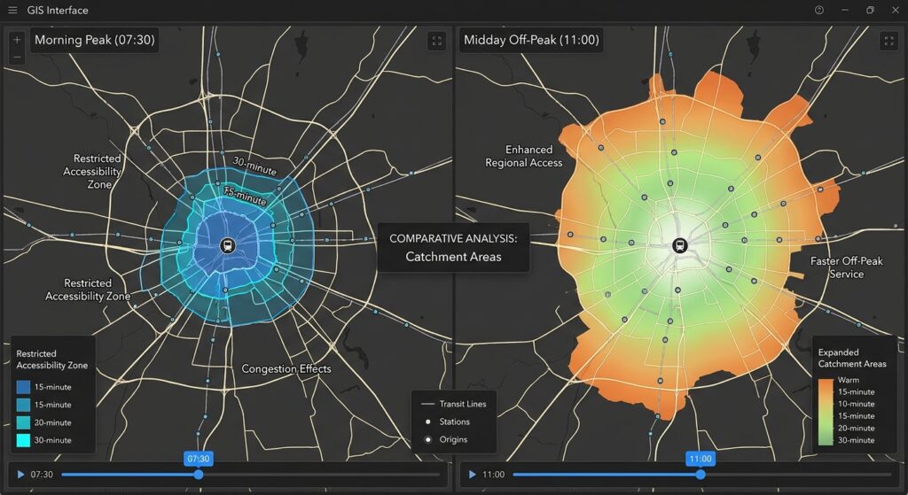
Public transit is inherently time-dependent. A journey that takes 35 minutes in the morning may require 55 minutes at midday because departure frequencies, transfers, and available services differ.
A useful accessibility study should compare several explicitly defined time scenarios rather than calculate a single static travel-time surface.
For example, an urban planning project might use:
| Scenario | Example departure time | Planning question |
|---|---|---|
| Morning peak | Tuesday, 7:30 AM | Can residents reach work or a clinic during the morning commute? |
| Off-peak | Tuesday, 11:00 AM | How accessible are services for people traveling outside commuting hours? |
| Evening peak | Tuesday, 5:30 PM | Can residents return home or reach evening services? |
| Weekend | Saturday, 10:00 AM | How does weekend service affect access to healthcare, shopping, or recreation? |
These are illustrative scenarios, not assumptions about any particular transit system. Select real analysis dates and local times that match your study objectives and the validity dates of the GTFS feed.
Configure each scenario consistently
For each run:
- Set a date when the relevant transit service is operating.
- Set the departure time or arrival deadline.
- Use consistent walking assumptions and transfer preferences.
- Retain the same study boundary and destination dataset.
- Record the routing configuration and feed version.
- Export results with a clear scenario identifier, such as
peak_0730oroffpeak_1100.
A depart-at analysis asks how far a traveler can get after leaving at a given time. An arrive-by analysis asks when a traveler must leave to reach a destination by a specified time. An arrival deadline is often useful for evaluating access to a job before the start of a shift or access to a healthcare appointment.
Do not replace scheduled public transit with straight-line distances or a constant road speed when comparing time scenarios. Waiting time, available departures, transfers, and service-calendar rules are part of the travel-time calculation.
6. Step 4 — Generate multimodal travel-time catchments
A public transport catchment is the area or set of destinations reachable within a selected travel-time threshold. Examples include a 15-minute, 30-minute, or 45-minute catchment.
Unlike a circular buffer around a bus stop, a timetable-aware transit catchment accounts for the time required to reach stops, wait for services, transfer, ride transit, and walk to destinations.
Door-to-door time can be represented conceptually as:
[
T_{\text{total}} =
T_{\text{access walk}} +
T_{\text{initial wait}} +
T_{\text{transit}} +
T_{\text{transfer}} +
T_{\text{egress walk}}
]
Here, transfer time includes relevant transfer walking and waiting. The routing engine normally calculates these components as part of the itinerary; do not add them again to its reported total journey time.
6.1 Generate isochrones
An isochrone shows the area reachable from an origin within a specified period.
For example, from a neighborhood center, generate 15-, 30-, and 45-minute public transport catchments. If the engine supports temporal accessibility, repeat the calculation at the morning peak and off-peak departures.
In QGIS with a compatible OpenTripPlanner workflow, use an isochrone or temporal accessibility tool. In ArcGIS Pro, use a transit-enabled Service Area analysis.
Recommended outputs include:
- A 15-minute catchment.
- A 30-minute catchment.
- A 45-minute catchment.
- A comparable set of outputs for each selected time scenario.
The resulting catchments are generally irregular because roads, transit routes, service frequency, transfers, and network connectivity determine which locations can be reached.
Important: An isochrone from one origin is not sufficient to establish equitable access across an entire city. Accessibility may vary considerably from one residential block to another. For neighborhood-level comparisons, calculate travel times from multiple origins or use a consistent population grid.
6.2 Calculate an origin-destination travel-time matrix
A travel-time matrix records the minimum modeled journey time between each selected origin and destination.
For an access-to-employment study, origins could be residential neighborhood centroids or population-grid cells, while destinations are employment locations. For healthcare access, origins represent residential populations and destinations represent clinics, hospitals, or other relevant service facilities.
A simplified matrix might look like this:
| Origin | Destination | Morning travel time | Off-peak travel time |
|---|---|---|---|
| Neighborhood A | Hospital 1 | 28 min | 24 min |
| Neighborhood A | Hospital 2 | 47 min | 39 min |
| Neighborhood B | Hospital 1 | 41 min | 36 min |
| Neighborhood B | Hospital 2 | 33 min | 31 min |
These are illustrative values. Real outputs must come from the selected routing engine, feed, and time scenario.
The matrix allows planners to distinguish the geographic proximity of a destination from its actual accessibility by public transport.
6.3 Calculate cumulative-opportunity accessibility
A common accessibility indicator is the number of opportunities reachable within a travel-time threshold.
For origin (i) and threshold (T):
[
A_i(T) =
\sum_j O_j , I(t_{ij} \leq T)
]
Where:
- (A_i(T)) is the number or weighted amount of opportunities accessible from origin (i).
- (O_j) is the number of opportunities at destination (j), such as jobs or healthcare capacity.
- (t_{ij}) is the modeled door-to-door travel time between origin (i) and destination (j).
- (I(t_{ij}\leq T)) equals 1 when the destination is reachable within the threshold and 0 otherwise.
This method can quantify the number of jobs accessible within 30 minutes or the amount of healthcare capacity reachable within 45 minutes.
7. Applied example — Evaluating equitable access to jobs and healthcare
Suppose a city planning team wants to determine whether lower-income neighborhoods have poorer public transport access to employment and healthcare than other neighborhoods.
The analysis uses four inputs:
- Residential origins with population and income indicators.
- Job centers or healthcare facilities with an opportunity measure.
- A GTFS-based routing model combining transit schedules and pedestrian access.
- Morning peak and off-peak origin-destination matrices.
The aim is not merely to map where transit stops exist. It is to evaluate whether people can reach useful destinations within a reasonable amount of time.
7.1 Prepare the datasets
Create the following layers:
origins.gpkg: containsorigin_id,population,low_income_share, and neighborhood geometry.destinations.gpkg: containsdest_id,opportunities, and destination geometry.od_peak.csv: contains origin-destination pairs and morning peak travel times.od_offpeak.csv: contains the comparable off-peak travel times.
For employment, opportunities could represent the number of jobs at each destination. For healthcare, it might represent the number of facilities, available clinicians, or hospital beds, depending on the planning objective and the available data.
The matrix files should use at least these fields:
origin_id,destination_id,total_minutes
A001,H001,28
A001,H002,47
A002,H001,41
A002,H002,33
These are sample rows. total_minutes should represent the full modeled journey, including the relevant walking, waiting, riding, and transfer components.
7.2 Calculate accessible opportunities with Python
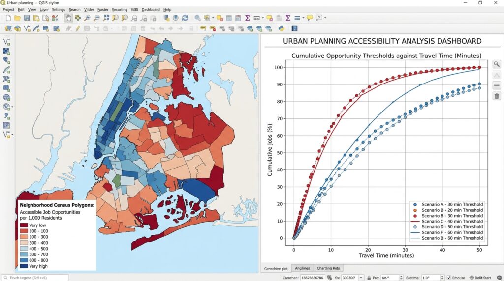
Use the following script to calculate how many opportunities can be reached within 45 minutes. It aggregates destination opportunities for each residential origin, creates accessible-opportunity rates per 1,000 residents, and saves a GIS layer for mapping.
Install the required libraries:
python -m pip install pandas geopandas numpySave this as calculate_accessibility.py:
import pandas as pd
import geopandas as gpd
import numpy as np

# -------------------------------------------------
# Input datasets
# -------------------------------------------------

ORIGINS_FILE = "origins.gpkg"
DESTINATIONS_FILE = "destinations.gpkg"

PEAK_MATRIX = "od_peak.csv"
OFFPEAK_MATRIX = "od_offpeak.csv"

TIME_THRESHOLD = 45


# -------------------------------------------------
# Calculate cumulative-opportunity accessibility
# -------------------------------------------------

def calculate_accessibility(matrix_file, period):
    """
    Sum destination opportunities reachable from each origin
    within the selected door-to-door travel-time threshold.

    Required matrix fields:
        origin_id, destination_id, total_minutes

    Required destination fields:
        dest_id, opportunities

    Required origin fields:
        origin_id, population
    """

    origins = gpd.read_file(ORIGINS_FILE)
    destinations = gpd.read_file(DESTINATIONS_FILE)

    # Read identifiers as strings to avoid mismatched IDs.
    matrix = pd.read_csv(
        matrix_file,
        dtype={
            "origin_id": str,
            "destination_id": str
        }
    )

    origins["origin_id"] = origins["origin_id"].astype(str)
    destinations["dest_id"] = destinations["dest_id"].astype(str)

    matrix["total_minutes"] = pd.to_numeric(
        matrix["total_minutes"],
        errors="coerce"
    )

    destinations["opportunities"] = pd.to_numeric(
        destinations["opportunities"],
        errors="coerce"
    ).fillna(0)

    origins["population"] = pd.to_numeric(
        origins["population"],
        errors="coerce"
    )

    # Retain the minimum travel time for each OD pair.
    # This prevents duplicate alternative itineraries from
    # counting the same destination more than once.
    matrix = (
        matrix
        .dropna(subset=["total_minutes"])
        .groupby(
            ["origin_id", "destination_id"],
            as_index=False
        )["total_minutes"]
        .min()
    )

    # Select destinations reachable within the time limit.
    reachable = matrix.loc[
        matrix["total_minutes"] <= TIME_THRESHOLD
    ].merge(
        destinations[["dest_id", "opportunities"]],
        left_on="destination_id",
        right_on="dest_id",
        how="inner"
    )

    # Sum opportunity counts for every residential origin.
    accessibility = (
        reachable
        .groupby("origin_id")["opportunities"]
        .sum()
        .rename(f"opp_{period}")
    )

    output = origins.merge(
        accessibility,
        left_on="origin_id",
        right_index=True,
        how="left"
    )

    metric = f"opp_{period}"

    # Origins with no reachable destinations receive zero.
    output[metric] = output[metric].fillna(0)

    # Normalize for differences in neighborhood population.
    output[f"opp_per_1000_{period}"] = (
        output[metric]
        / output["population"].replace(0, np.nan)
        * 1000
    )

    return output


# -------------------------------------------------
# Calculate peak and off-peak accessibility
# -------------------------------------------------

peak = calculate_accessibility(
    PEAK_MATRIX,
    "peak"
)

offpeak = calculate_accessibility(
    OFFPEAK_MATRIX,
    "offpeak"
)

# Combine the two outputs by origin.
peak_attributes = peak.drop(
    columns="geometry"
)

offpeak_attributes = offpeak.drop(
    columns="geometry"
)

result = peak.merge(
    offpeak_attributes[
        [
            "origin_id",
            "opp_offpeak",
            "opp_per_1000_offpeak"
        ]
    ],
    on="origin_id",
    how="left"
)

# Calculate absolute change and percentage change.
result["opp_change_offpeak_minus_peak"] = (
    result["opp_offpeak"] - result["opp_peak"]
)

result["opp_pct_change"] = np.where(
    result["opp_peak"] > 0,
    (
        result["opp_change_offpeak_minus_peak"]
        / result["opp_peak"]
    ) * 100,
    np.nan
)

# Export the results to GeoPackage.
result.to_file(
    "accessibility_results.gpkg",
    layer="neighborhood_accessibility",
    driver="GPKG",
    index=False
)

# Export a flat table for summaries and reporting.
result.drop(columns="geometry").to_csv(
    "accessibility_results.csv",
    index=False
)

print("Accessibility analysis completed.")
print("Outputs: accessibility_results.gpkg")
print("         accessibility_results.csv")
The script assumes the two matrix files were generated using the same origin and destination identifiers, study area, opportunity dataset, and modeling assumptions apart from the departure-time scenario.
In QGIS, symbolize opp_per_1000_peak and opp_per_1000_offpeak to display accessible opportunities by neighborhood. Use a consistent classification method and comparable class breaks when comparing the maps.
A low value indicates that the origin has relatively few opportunities reachable within the specified period. A high value indicates that more opportunities are accessible under the modeled conditions.
7.3 Interpret the results from an equity perspective
Suppose the morning peak map shows that lower-income neighborhoods can reach fewer jobs within 45 minutes than other residential areas. This may indicate a disadvantage in access to employment opportunities.
However, the pattern should not automatically be attributed to transit service alone. Neighborhood differences may also reflect the geographic distribution of jobs, residential density, service availability, street connectivity, and the characteristics of the population.
A defensible interpretation should consider several indicators:
Accessible opportunities: Count jobs or healthcare resources reachable within 30, 45, or 60 minutes.
Population-weighted accessibility: Assess how many residents live in areas with low accessibility rather than relying only on neighborhood averages.
Temporal variation: Compare peak and off-peak results to identify neighborhoods with limited service outside commuting hours.
Service coverage: Investigate whether residents have safe, usable walking connections to public transport stops.
Distributional equity: Compare accessibility across income groups or neighborhood deprivation categories, using a consistent spatial and statistical method.
For healthcare, consider whether the available destinations provide the relevant service. A nearby clinic may not offer emergency care, specialist services, or sufficient capacity. Counting all healthcare facilities equally may therefore misrepresent access to the care residents need.
7.4 Turn results into planning recommendations
The outputs can support decisions such as:
- Improving walking connections to existing stops.
- Reviewing service frequencies on routes serving poorly connected neighborhoods.
- Adjusting transfers and timetables to reduce excessive waiting.
- Identifying areas where new transit services may improve access to jobs or essential services.
- Testing how proposed routes or service changes alter accessibility before implementation.
The strongest workflow compares a documented baseline with one or more plausible interventions. For example, a planner might test the change in the number of jobs reachable within 45 minutes if a connecting service operated more frequently or if a new link improved pedestrian access to a major station.
The results should be interpreted as modeled accessibility, not a guarantee of actual journey performance. Scheduled feeds may omit disruptions, overcrowding, unreliable travel times, or other conditions that affect passenger experience.
8. Limitations and quality assurance
Before using accessibility maps to guide public investment, check the following issues.
Timetable accuracy
Confirm that the selected GTFS feed covers the chosen dates, includes all relevant operators, and correctly represents weekday, weekend, and holiday service. A routing engine cannot identify a service that is missing from its source feed.
Pedestrian-network completeness
OSM coverage varies by location. Missing footpaths, station entrances, crossings, or pedestrian restrictions can make accessible destinations appear unreachable. Inspect the walking connections around stops and major trip generators.
Walking speed and mobility constraints
A single walking speed does not represent every traveler. Older adults, wheelchair users, and people with mobility limitations may experience different journey times or lack accessible routes entirely. Where possible, conduct separate analyses with relevant walking speeds, accessibility constraints, and assumptions about stairs, elevators, crossings, and station access.
Transfers and waiting time
Verify that the routing engine interprets the GTFS schedule and transfer data as intended. Two destinations that are close in straight-line distance can have very different journey times because of service frequency and transfer patterns.
Spatial aggregation
Neighborhood centroids may not represent all residents equally, particularly in large or irregularly shaped neighborhoods. For more detailed analysis, use residential address points, population-weighted grid cells, or a set of origins that reflects where people actually live.
Model limitations
Results from OTP, ArcGIS, and other transit-routing systems may differ because of differences in configuration, transfer rules, network topology, walking assumptions, and schedule interpretation. Document the engine, version, settings, data sources, and analysis date to support reproducibility.
9. Summary and practical takeaways
Multimodal accessibility modeling with GTFS in GIS combines public transport schedules with pedestrian and street networks to estimate the places travelers can reach within a given time. It goes beyond road distance or circular buffers by incorporating departure times, service calendars, waiting, transfers, transit travel, and access and egress walking.
For an applied urban planning project, begin with reliable GTFS and OSM data, validate the feed, construct a timetable-aware routing network, and run separate peak and off-peak scenarios. Generate catchments or origin-destination matrices, calculate the number of jobs or services accessible within specified travel times, and map the results alongside population and socioeconomic indicators.
The principal planning value is the ability to measure accessibility as an outcome rather than treating the presence of a road or transit stop as sufficient evidence of mobility.
A carefully validated accessibility model can reveal which neighborhoods have limited access to essential destinations, how those gaps change throughout the day, and which transportation interventions are worth investigating further.