

Estimating Building Energy Consumption Using 3D City Models (CityGML) in QGIS
Introduction

Urban energy planning increasingly relies on three-dimensional representations of buildings rather than conventional two-dimensional maps. With the development of urban digital twins, planners can combine building geometry, construction characteristics, meteorological observations, and energy data to investigate how buildings perform within their surrounding environment.
The Open Geospatial Consortium’s (OGC) City Geography Markup Language (CityGML) standard provides a structured way to represent, exchange, and manage virtual 3D city models. Depending on the dataset’s level of detail (LoD), these models can contain building footprints, roof structures, façades, semantic surface classifications, and additional building attributes. CityGML supports applications including urban planning, infrastructure management, and environmental and energy simulations.
Combining 3D City Models CityGML Building Energy QGIS workflows allows spatial analysts to estimate heating demand, examine solar exposure, identify inefficient building geometries, and map areas with opportunities for energy improvements.
However, a 3D city model does not automatically contain the information required to calculate actual energy consumption. Geometry provides the spatial foundation, while construction materials, thermal transmittance, occupancy, ventilation, weather, and heating-system efficiency determine the physical energy model.
This tutorial develops a reproducible workflow using QGIS, CityGML-compatible data preparation tools, GRASS GIS, and optional urban climate modelling extensions. The objective is to create building-level estimates of thermal energy demand and solar potential and visualize the resulting indicators in a 3D urban environment.
1. Data Preparation: Importing CityGML into QGIS
Before calculating building energy indicators, prepare a consistent dataset containing building geometry, identifying attributes, and the physical parameters needed for modelling.
1.1 Required datasets
The minimum inputs depend on the intended level of accuracy. A preliminary urban screening model can use building footprints and heights, whereas a detailed thermal model requires semantic surfaces and building-performance information.
| Dataset | Essential attributes | Analytical purpose |
|---|---|---|
| 3D building model | Building ID, geometry, height, LoD | Building shape and volume |
| Roof surfaces | Roof geometry, slope, orientation | Solar radiation and PV potential |
| Wall surfaces | Wall geometry, material class | Transmission heat loss |
| Building properties | Floor area, floor count, construction type | Thermal demand estimates |
| Window information | Window area, glazing type | Heat loss and solar gains |
| Weather data | Heating degree days, irradiance, temperature | Annual demand estimation |
| Terrain and surroundings | Elevation, neighbouring buildings, trees | Shading and local exposure |
| Energy attributes | U-values, ventilation rate, system efficiency | Energy calculations |
CityGML distinguishes semantic surface types such as RoofSurface, WallSurface, and GroundSurface. These classifications are valuable because a roof and an exterior wall can have different thermal properties and receive different amounts of solar radiation.
Use the highest available geometric detail that is justified by the project. A model representing simple building blocks is adequate for neighbourhood-scale screening, but it cannot reliably represent complex roof angles, recessed façades, or individual window areas.
1.2 Importing CityGML files
CityGML is an XML-based geospatial format, but its nested application schema and 3D geometry structures mean that opening a file directly in QGIS does not always produce usable, semantically complete building layers. GDAL’s standard GML driver has limitations when handling application-schema structures and complex feature representations.
Choose one of the following import approaches.
Option A: Convert CityGML to CityJSON
For a file-based workflow, the open-source citygml-tools utility can convert CityGML XML files into CityJSON.
-
Install Java 11 or a compatible newer version supported by the selected tool release.
-
Download a compatible
citygml-toolsrelease from its official project resources. -
Open a command prompt in the utility’s directory.
-
Convert the source file:
citygml-tools to-cityjson buildings.gmlThe tool creates a CityJSON file from the input when the file is supported.
Next, install CityJSON Loader from the QGIS Python Plugins Repository. Use Vector → CityJSON Loader → Load CityJSON to import the model. The plugin supports loading CityJSON features into QGIS and provides access to semantic surfaces and levels of detail. Check compatibility with your installed QGIS version before installation.
Inspect the imported layers before continuing. Confirm that building identifiers, surface classifications, coordinates, and elevation values have been preserved.
Option B: Use a CityGML database
For large datasets or repeatable citywide workflows, a spatial database is often more suitable.
The 3D City Database provides CityGML import and export capabilities with PostgreSQL/PostGIS support. The QGIS 3DCityDB Tools plugin connects QGIS to supported 3D City Database 4.x schemas and can load building features, including supported levels of detail, as accessible layers. This is a version-specific workflow; confirm that the dataset and database versions are compatible.
Once loaded, use PostGIS to filter the study area, select relevant surface types, and export working subsets into GeoPackage or SpatiaLite for local analysis.
Where does SpatiaLite fit?
SpatiaLite is useful for lightweight local storage and SQL-based filtering, but it should not be treated as an automatic converter of arbitrary CityGML documents. First extract and validate the required geometry and attributes with a compatible importer, then store the resulting analytical layers in SpatiaLite or GeoPackage.
1.3 Standardize the coordinate system
All area, height, and volume calculations must use consistent units.
In QGIS:
-
Inspect the source dataset’s coordinate reference system (CRS).
-
Reproject the analytical layers to an appropriate projected CRS with metre-based coordinates.
-
Confirm that building elevations are in metres.
-
Check that the terrain, roof, wall, and footprint layers overlap correctly.
-
Compare sample building measurements with known or independently calculated dimensions.
Do not simply assign a new CRS to a dataset with incorrect coordinates. Use an actual coordinate transformation when converting between reference systems.
Save the validated layers in a working GeoPackage, with separate tables for building footprints, roof surfaces, wall surfaces, and calculated attributes.
2. Extracting Building Volumes, Surface Areas, and Ratios
The next stage transforms geometric objects into indicators that can be used in a thermal energy model.
2.1 Calculate building floor area and volume
Start with a unique building identifier and a footprint layer.
Use the QGIS Field Calculator to create a footprint_m2 field:
$areaThis expression calculates the area according to QGIS’s project measurement settings. Check the ellipsoid, CRS, and units before interpreting the result as square metres.
For conditioned floor area, the footprint area alone is insufficient for multistorey buildings. If the footprint is representative of every storey, a preliminary estimate is:
where:
-
\(A_f\) is total floor area in square metres;
-
\(A_{\text{footprint}}\) is the building footprint area;
-
\(N_f\) is the number of storeys.
Exclude unconditioned spaces and adjust for varying floor plates when data are available.
For building volume, prefer a validated volume attribute or calculate the volume from a closed, valid 3D solid using a geometry-processing engine that supports volumetric calculations.
If only a footprint and an estimated mean height are available, use:
This approximation assumes a simplified building form. It may be inaccurate for pitched roofs, podiums, stepped structures, voids, and buildings with substantially different upper-floor footprints.
A CityGML building solid, semantic surface geometry, and an attribute describing measured height are not interchangeable. A measured height is not itself a volume.
2.2 Derive roof and wall areas
Use the semantic surface classifications to separate roofs from façades.
For a flat roof represented in plan, its planimetric area may approximate its physical area. For a planar sloping roof with slope angle \(\theta\), its physical surface area can be estimated from the horizontal projected area:
The equation assumes a single planar surface and a consistent slope angle.
For buildings with multiple roof facets, calculate each facet separately and sum the results. Use actual 3D face areas where possible, especially for irregular roof geometries.
Similarly, calculate exterior wall areas from the individual façade surfaces. Subtract window and door openings when they are represented separately and the thermal model requires opaque-wall area.
Important: QGIS’s ordinary $area measurement is not a general-purpose 3D surface-area calculation for sloping faces. Do not assume that the projected area of a roof polygon equals its actual surface area.
2.3 Calculate surface-to-volume and wall-to-floor ratios
Two useful geometric indicators are:
Envelope surface-to-volume ratio
Here, \(A_{\text{env}}\) is the total relevant exterior envelope area and \(V\) is the conditioned building volume.
A relatively high ratio indicates more envelope area through which heat may be transferred per unit of enclosed volume. All other factors being equal, this can increase heating or cooling loads.
Wall-to-floor area ratio
This ratio can help compare buildings of different sizes. Define clearly whether exposed walls include party walls and whether window areas are included in the numerator.
For improved analysis, maintain separate fields for opaque walls, windows, roofs, and ground-contact surfaces. Each can have a different thermal transmittance.
3. Calculating Solar Radiation on Roof Surfaces
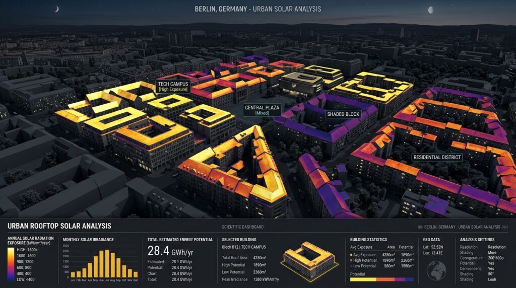
Solar exposure influences rooftop photovoltaic potential and can contribute to building heating gains through windows and other solar-accessible elements. It also interacts with urban shading, roof orientation, and local microclimate.
QGIS supports solar-related workflows through GRASS GIS and complementary urban climate modelling tools.
3.1 Prepare the 3D surface model
For an initial urban solar analysis, create a digital surface model (DSM) representing roof heights and surrounding obstructions.
The DSM should capture:
-
Roof ridges and changes in elevation.
-
Adjacent buildings that cast shadows.
-
Relevant tree canopy and terrain features.
-
A consistent horizontal and vertical reference system.
Rasterize suitable 3D surface data or generate a surface using appropriate interpolation tools. Select a cell size that reflects the detail in the source geometry. A coarse grid can smooth out narrow roofs and ridges, while an excessively fine grid increases processing time without necessarily improving accuracy.
Do not derive a DSM from footprints with uniform assumed heights when the analysis depends on individual roof slopes.
3.2 Choose the solar radiation method
There are two practical approaches.
Approach A: GRASS GIS r.sun
The GRASS r.sun module estimates direct, diffuse, and reflected solar radiation using an elevation surface, slope, aspect, atmospheric parameters, and solar geometry. It can account for terrain-related shading.
In QGIS, open the Processing Toolbox and locate the GRASS solar radiation algorithm.
Prepare the necessary elevation, slope, and aspect rasters and configure:
-
Latitude and longitude for the study area.
-
The elevation model and surface orientation inputs.
-
Atmospheric and diffuse-radiation parameters where available.
-
The date, time, or irradiation calculation settings.
-
The output raster resolution and extent.
Run an initial calculation to inspect the radiation pattern. For annual irradiation, use a supported cumulative or repeated time-step workflow and combine the results using consistent units and assumptions.
r.sun is a raster-based surface model. Applying it to individual urban roofs requires careful construction of the surface model and evaluation of how buildings and vertical façades are represented. It should not automatically be interpreted as a complete façade-by-façade building radiation model.
Approach B: UMEP and SEBE
For detailed built-environment radiation studies, consider UMEP for QGIS. Its modelling framework includes tools for urban climate and radiation analyses; its associated SEBE workflow supports solar irradiation calculations for urban surfaces, including roofs and walls.
Use a version compatible with your QGIS installation, then prepare the required urban geometry, DSM and meteorological inputs. Follow the selected model’s requirements for vegetation, building obstructions, surface orientations, and radiation data.
This approach is particularly useful when the objective is to compare roofs that have different slopes, azimuths, and shading conditions.
3.3 Interpret the solar output
For every roof or raster cell, obtain a solar irradiation value.
Annual irradiation is commonly reported as:
Use this quantity to identify suitable roof areas and compare buildings.
For a simplified photovoltaic estimate:
where:
-
\(E_{\text{PV}}\) is estimated annual electricity generation in kWh;
-
\(A_{\text{usable}}\) is usable panel area in square metres;
-
\(\eta_{\text{PV}}\) is panel conversion efficiency;
-
\(PR\) is the system performance ratio.
Account for roof obstructions, access pathways, setbacks, panel spacing, and additional shading before interpreting this value as installable PV potential.
Solar irradiation should not be subtracted directly from total building heat loss. Only the portion of solar energy that enters the conditioned building, after glazing and shading effects, can contribute to useful internal gains.
4. Estimating Thermal Heat Loss
Geometric analysis becomes an energy model only when envelope surfaces are assigned plausible thermal properties.
4.1 Create a building thermal properties table
Create a table joined to the building layer using building_id. Include the following fields:
| Field | Unit | Purpose |
|---|---|---|
U_wall |
W/m²K | Wall thermal transmittance |
U_roof |
W/m²K | Roof thermal transmittance |
U_window |
W/m²K | Window thermal transmittance |
U_ground |
W/m²K | Ground-contact envelope transmittance |
n_air |
h⁻¹ | Air-change rate |
HDD |
K·days/year | Annual heating degree days |
eta_heat |
0–1 | Heating system efficiency |
floor_area |
m² | Conditioned floor area |
volume |
m³ | Conditioned building volume |
Obtain values from building surveys, available energy certificates, construction records, applicable technical standards, or clearly documented typology-based assumptions.
Do not assign thermal properties solely from building height, footprint size, or roof colour. Those variables are not reliable substitutes for construction data.
4.2 Calculate the transmission heat-loss coefficient
For a simplified steady-state envelope calculation:
where:
-
\(H_{\text{tr}}\) is the transmission heat-loss coefficient in W/K;
-
\(U_i\) is the thermal transmittance of envelope component \(i\), in W/m²K;
-
\(A_i\) is the area of that component in m².
For example:
where the subscripts represent walls, roof, ground-contact surfaces, and windows.
Thermal bridges can also contribute to heat transfer. For a more detailed estimate, include linear thermal-bridge coefficients and junction lengths.
4.3 Estimate ventilation and infiltration losses
If the air-change rate is expressed in air changes per hour, a simplified ventilation heat-loss coefficient can be approximated by:
where:
-
\(H_{\text{ve}}\) is in W/K;
-
\(n\) is the air-change rate in h⁻¹;
-
\(V\) is the conditioned volume in m³.
The coefficient of approximately 0.33 represents the volumetric heat capacity of air in Wh/(m³·K), under typical assumptions. The formulation assumes a simplified air-volume flow and does not account fully for heat recovery or more complex ventilation behaviour.
The total simplified heat-loss coefficient is:
This represents the rate of heat loss per degree of indoor–outdoor temperature difference.
4.4 Estimate annual heating demand
Using annual heating degree days, the gross annual space-heating requirement can be screened with:
where:
-
\(Q_{\text{gross}}\) is expressed in kWh of thermal energy per year;
-
\(H\) is in W/K;
-
\(HDD\) is in kelvin-days per year;
-
24 converts days into hours;
-
1,000 converts Wh into kWh.
This formula estimates a simplified gross heating requirement before useful internal and solar gains, controls, intermittent occupancy, and other effects are fully considered.
For a more complete model, subtract the useful fraction of solar and internal gains:
Here, \(\eta_g\) represents the fraction of gains that can be used to offset heating demand. This simplified expression is a screening approximation, not a substitute for a calibrated building energy simulation.
Keep annual thermal demand separate from energy purchased. For a heating system with an efficiency or seasonal performance factor represented by \(\eta_{\text{heat}}\):
Use an appropriate seasonal coefficient of performance for heat pumps rather than treating them like conventional combustion boilers.
Cooling loads require a separate calculation that accounts for cooling degree conditions, solar gains, internal loads, ventilation, thermal storage, and system controls. Heating degree days alone cannot predict total annual energy consumption.
4.5 Implement the equations in QGIS
Join the relevant building measurements and thermal parameters to a single building-level table.
In the Field Calculator, create a field called h_trans_WK using an expression such as:
"U_wall" * "wall_area" +
"U_roof" * "roof_area" +
"U_window" * "window_area" +
"U_ground" * "ground_area"
This expression assumes the areas have already been correctly calculated, the U-values use W/m²K, and each surface is represented exactly once.
Calculate ventilation losses:
0.33 * "n_air" * "volume"Create h_total_WK:
"h_trans_WK" + "h_vent_WK"Finally, calculate gross annual heating demand:
"h_total_WK" * "HDD" * 24 / 1000The output is an estimate in kWh of thermal energy per year.
Add fields for the model version, input-data source, and assumption category. Buildings with missing U-values, unknown floor areas, or incomplete geometry should be flagged rather than assigned arbitrary values without documentation.
5. Visualizing Energy Consumption Tiers in 3D
QGIS native 3D map views let analysts explore building geometry and attribute-driven styling within a three-dimensional scene. Vector layers can use 3D renderers, including height or extrusion settings that are configured through the layer’s 3D properties.
5.1 Prepare the energy results layer
Join the completed energy table to the building footprint layer using building_id.
Useful output indicators include:
-
annual_heat_kwh: estimated yearly space-heating demand. -
heat_kwh_m2: estimated demand per square metre of floor area. -
heat_loss_WK: envelope and ventilation heat-loss coefficient. -
solar_kwh_m2: annual solar irradiation on the roof. -
pv_kwh: estimated annual photovoltaic output.
Per-square-metre demand is especially important. A large commercial building might use more energy in total than a small house simply because it is larger. Normalizing by conditioned floor area helps identify relatively energy-intensive buildings.
5.2 Configure the 3D renderer
Open Layer Properties → 3D View and enable the appropriate 3D renderer.
For footprint-based buildings, use the available elevation and extrusion settings to display building height. If the source layer already contains valid 3D building geometry, use that geometry instead of generating an additional extrusion.
Next:
-
Open the layer’s symbology settings.
-
Choose graduated styling based on
heat_kwh_m2. -
Define meaningful low, medium, high, and very high demand classes.
-
Open View → 3D Map Views → New 3D Map View.
-
Adjust the camera, terrain, lighting, and visible layers.
-
Compare the mapped demand classes with roof irradiation and surrounding building density.
Use consistent class thresholds across different neighbourhoods when direct comparison is required. Quantile classes are helpful for exploring relative rankings, but they can make buildings with quite different energy values appear comparable.
For a more informative scene, create a separate roof layer styled by annual irradiation while keeping the building layer styled by energy demand. Avoid representing two unrelated numerical indicators through one colour ramp.
[Image 1: 3D city model rendered in QGIS color-coded by estimated building energy loss]
Alt Text: “QGIS 3D map view displaying extruded building footprints color-coded by solar radiation exposure and simulated energy consumption.”
Suggested caption: A 3D urban energy screening map combining estimated building heating demand with roof-level solar potential to identify priority buildings for energy efficiency upgrades and renewable energy installations.
5.3 Interpret the spatial patterns
Use the scene to investigate questions such as:
-
Do buildings with high envelope surface-to-volume ratios also have high heating demand per square metre?
-
Are buildings with poor roof solar exposure concentrated in narrow, shaded streets?
-
Which large roofs offer substantial PV potential?
-
Do older or poorly insulated building categories dominate estimated thermal demand?
-
Are high-demand buildings clustered near areas with limited solar access?
These patterns can guide field surveys and renovation prioritization. They should not be interpreted as proof of actual energy consumption without measured or independently modelled consumption data.
6. Validation, Uncertainty, and Model Limitations
The reliability of a 3D building energy estimate depends on geometry, thermal parameters, climate data, and modelling assumptions.
Start by comparing a sample of buildings with known floor areas, roof dimensions, and construction properties. Inspect invalid solids, duplicated surfaces, missing openings, incorrect storey counts, and vertical coordinate errors.
Next, test the sensitivity of results to uncertain parameters. For example, calculate demand under low, medium, and high plausible envelope U-values and air-change rates. If the ranking of energy-intensive buildings changes significantly, report that uncertainty.
Where available, compare results against utility consumption, energy certificates, site surveys, or calibrated building simulation outputs. Meter readings may include domestic hot water, cooking, appliances, or cooling, so make sure the comparison uses matching energy categories and reporting periods.
Finally, recognize the following limitations:
-
Simplified geometry may underestimate façade or roof area.
-
Unknown construction materials can produce large errors in heat-loss estimates.
-
A roof irradiation model does not independently determine building electricity demand.
-
Occupancy, thermostat settings, heating schedules, and system efficiency can substantially affect real consumption.
-
Urban shading can be misrepresented if trees or neighbouring structures are missing from the surface model.
Document these limitations directly in the output metadata. A transparent screening model is more useful than an apparently precise estimate with undocumented assumptions.
7. SEO Best Practices and Internal Linking
To strengthen this tutorial’s topical coverage, connect it with related GIS workflows that address complementary environmental and geometric questions.
Recommended internal links include:
| Suggested anchor text | Recommended destination |
|---|---|
| Extracting LiDAR canopy height models | /lidar-canopy-height-model-extraction/ |
| Urban Heat Island mapping with Landsat | /urban-heat-island-mapping-landsat-lst/ |
| Calculating building solar potential in QGIS | A related solar radiation tutorial |
| Processing CityGML files in QGIS | A CityGML data import and conversion guide |
Replace these example paths with the actual published URLs on your website.
The LiDAR article can explain how vegetation and canopy height affect urban shading inputs, while the Urban Heat Island mapping article can provide wider thermal context for neighbourhood-scale climate analysis. Landsat land surface temperature is not a direct measurement of indoor building temperature or energy consumption, so maintain that distinction when linking the topics.
Use the primary target keyword naturally in the introduction, one relevant subheading, and the conclusion. Include secondary keywords where they accurately describe the procedure rather than repeating them unnaturally.
Screenshots should show recognizable QGIS interface elements, relevant processing parameters, and interpretable outputs. The 3D visualization should communicate the specific relationship between solar exposure and estimated energy performance.
Conclusion: Estimating Building Energy Consumption Using 3D City Models (CityGML) in QGIS
Estimating building energy consumption with 3D CityGML data in QGIS combines geometric analysis, surface radiation modelling, thermal calculations, and three-dimensional visualization into a practical urban planning workflow.
The process begins by importing and validating CityGML data, extracting building dimensions and semantic surfaces, and calculating surface-to-volume ratios. Solar modelling then identifies roof exposure and shading patterns, while construction properties and weather data support simplified estimates of annual heating demand. Finally, QGIS’s 3D map view displays the resulting indicators for building-level comparison and neighbourhood prioritization.
The most important distinction is between geometric potential, estimated energy demand, and actual measured consumption. CityGML provides the spatial structure for the analysis, but trustworthy energy estimates require defensible thermal properties, climate inputs, system assumptions, and validation.
Used with these safeguards, 3D building energy modelling in QGIS can help urban planners identify inefficient building typologies, screen rooftop photovoltaic opportunities, and prioritize more detailed building-performance assessments before investing in major energy improvements.