
Geographic vs. Projected Coordinate Reference Systems (CRS) Explained Simply
Introduction: The Orange Peel Dilemma
When studying Geographic vs Projected CRS, imagine peeling an orange in one continuous piece and trying to lay that curved peel completely flat on a table without stretching or tearing it—it is physically impossible.
This classic orange peel analogy illustrates the central challenge of mapmaking and Spatial Data Infrastructure (SDI). The Earth is a three-dimensional, slightly squished sphere (an ellipsoid), but our computer screens, paper maps, and GIS layouts are two-dimensional flat surfaces. Flattening a 3D Earth onto a 2D surface without distorting shape, area, distance, or direction is mathematically impossible.
To bridge this dimensional gap, Geographic Information Systems (GIS) rely on Coordinate Reference Systems (CRS). Understanding the debate between Geographic vs Projected CRS is fundamental to mastering spatial analysis. If you have ever opened QGIS or ArcGIS only to find your layers floating miles apart, your area calculations returning wildly incorrect numbers, or your map looking oddly stretched, a CRS mismatch is almost certainly to blame.
This guide demystifies coordinate reference systems explained from the ground up, giving you the clarity needed to handle spatial data confidently.
Demystifying Geographic Coordinate Systems (GCS)
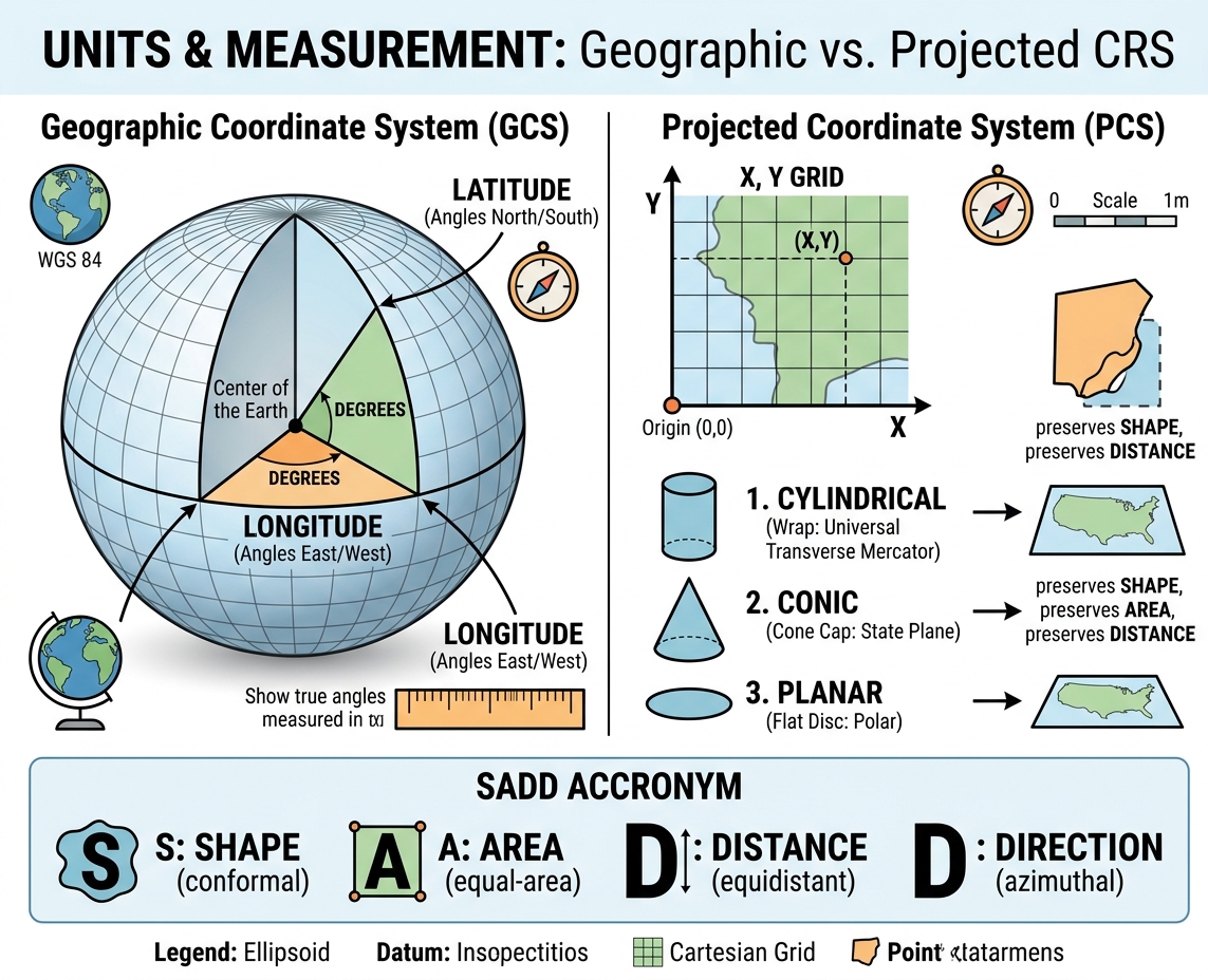
A Geographic Coordinate System (GCS) defines locations on a three-dimensional, spherical model of the Earth using angular units.
       North Pole
          |
     .---' '---.
    /     |     \
   |   Latitude  |  <-- Measured in Degrees North/South from Equator
   |------o------|  <-- Equator (0°)
   |  Longitude  |  <-- Measured in Degrees East/West from Prime Meridian
    \     |     /
     '---. .---'
          |
       South Pole
1. Latitude, Longitude, and Angular Measurements
Instead of using linear distances like meters or feet, a GCS measures positions using angles from the center of the Earth:
-
Latitude ($\phi$): Measures position north or south of the Equator (0° to 90°N or -90°S).
-
Longitude ($\lambda$): Measures position east or west of the Prime Meridian in Greenwich, England (0° to 180°E or -180°W).
Because these locations are measured from the center of a sphere, the unit of measurement is always angular units (decimal degrees or degrees, minutes, and seconds). When evaluating Geographic vs Projected CRS, the primary distinction in a GCS is that positions are defined using angular units rather than linear distances.
2. The Role of the Datum
A common misconception is that latitude and longitude are absolute physical lines painted on the Earth. In reality, they depend on a reference model called a datum.
A datum defines:
-
The precise shape and size of the Earth’s ellipsoid model.
-
The anchor point aligning the ellipsoid’s center with the Earth’s center of mass.
The most universal datum used globally today is WGS 84 (World Geodetic System 1984). It provides the reference frame for the Global Positioning System (GPS). If you record a coordinate point on your phone, it is almost certainly stored in WGS 84 (EPSG:4326).
3. Why Measuring Distance and Area in Degrees Fails
A core mistake students make when working with a GCS is running spatial analysis tools like Buffer, Calculate Area, or Distance Measure while their layer remains in decimal degrees.
Why is this a problem?
A degree is an angle, not a fixed physical length. While $1^\circ$ of latitude is always roughly 111 kilometers everywhere on Earth, $1^\circ$ of longitude shrinks dramatically as you move away from the Equator toward the poles:
-
At the Equator ($0^\circ$): $1^\circ$ of longitude $\approx 111 \text{ km}$
-
At $45^\circ$ Latitude: $1^\circ$ of longitude $\approx 78 \text{ km}$
-
At the North Pole ($90^\circ$): $1^\circ$ of longitude $= 0 \text{ km}$
If you attempt to calculate the area of a national park or create a 500-meter buffer in a Geographic CRS, your GIS software will try to apply that calculation to non-uniform, angular decimal degrees. The result? Completely skewed, useless values.
Demystifying Projected Coordinate Systems (PCS)
A Projected Coordinate System (PCS) takes the 3D angular coordinates of a Geographic CRS and mathematically flattens them onto a 2D Cartesian plane ($X, Y$ coordinate grid).
  Y (Northings)
   ^
   |       . Coordinate (X, Y)
   |
   |
   +-------------> X (Eastings)
 (0,0) Origin
Because a PCS is flat, it uses linear units such as meters, feet, or kilometers. This makes calculating lengths, perimeters, and surface areas straight forward using simple Euclidean geometry ($A = w \times h$ or $c^2 = a^2 + b^2$).
How Projections Work: The Three Developable Surfaces
To understand the core differences in Geographic vs Projected CRS, we must look at how map projections work. To project a curved surface onto a flat page, mathematicians project light rays through the Earth model onto a 2D shape that can be unrolled without stretching. These shapes are known as developable surfaces.
    1. CYLINDRICAL            2. CONIC               3. PLANAR (AZIMUTHAL)
      .------.                 /\                       ___
     |   ||   |               /  \                     /   \
     |  .||.  |              / .  \                   |  o  |
     |   ||   |             /______\                   \___/
      '------'              (Cone Cap)                (Flat Disc)
  Best for World Maps    Best for Mid-Latitudes      Best for Polar Regions
-
Cylindrical Projections:
-
Concept: Wrap a sheet of paper around the Earth like a cylinder.
-
Best For: Global maps or north-south strips along the line of tangency.
-
Example: Mercator, Transverse Mercator.
-
-
Conic Projections:
-
Concept: Place a cone over the Earth, touching along one or two lines of latitude (standard parallels).
-
Best For: Mid-latitude regions with broad east-west extents (e.g., the contiguous United States, Russia, or Europe).
-
Example: Lambert Conformal Conic, Albers Equal Area.
-
-
Planar / Azimuthal Projections:
-
Concept: Touch a flat disc against a single point on the Earth (usually one of the poles).
-
Best For: Polar navigation and hemispheric views.
-
Example: Polar Stereographic, Orthographic.
-
Universal Projection Systems: UTM and State Plane
Universal Transverse Mercator (UTM)
Rather than projecting the whole planet at once (which creates massive edge distortion), the UTM system divides the Earth into 60 longitudinal zones, each spanning $6^\circ$ of longitude.
-
Each zone uses a customized Secant Transverse Mercator projection centered on its own central meridian.
-
Distortion is kept under 0.04% within each zone.
-
Units are measured in meters using Eastings (X-axis) and Northings (Y-axis).
-
Example: UTM Zone 37N covers parts of East Africa, while UTM Zone 10N covers western North America.
State Plane Coordinate System (SPCS)
Used primarily in the United States, SPCS divides states into even smaller zones to minimize distortion to less than 1 part in 10,000. Larger states use multiple zones—for instance, California has 6 zones. Conic projections are used for east-west aligned zones, while Transverse Mercator projections are used for north-south zones.
The Distortion Trade-Off: Remembering SADD
Because you cannot flatten a 3D sphere without distortion, every map projection represents a compromise. In any Geographic vs Projected CRS conversion, a projection can preserve some metric properties, but only at the expense of others.
An easy way to remember these trade-offs is the SADD acronym:
            +-------------------------------------+
            |        THE SADD PROPERTIES          |
            +-------------------------------------+
            |  S  -->  Shape (Conformal)          |
            |  A  -->  Area (Equal-Area)          |
            |  D  -->  Distance (Equidistant)     |
            |  D  -->  Direction (Azimuthal)      |
            +-------------------------------------+
1. Shape (Conformal Projections)
-
Preserves: Local angles and shapes of small areas.
-
Distorts: Relative size/area as you move away from standard parallels.
-
Classic Example: The Mercator projection. While famous for keeping lines of constant compass bearing straight (ideal for marine navigation), it distorts area near the poles. Greenland appears the same size as Africa on a Mercator map, even though Africa is actually 14 times larger!
2. Area (Equal-Area / Equivalent Projections)
-
Preserves: Relative size and land surface area across the entire map.
-
Distorts: Local shapes and angles (lands look stretched or squished).
-
Classic Example: The Gall-Peters or Albers Equal Area Conic projections. Excellent for thematic density mapping, agriculture, and forestry management.
3. Distance (Equidistant Projections)
-
Preserves: True scale along specific selected lines or outward from a single central point.
-
Distorts: Distance across non-selected lines, along with shapes and areas elsewhere.
-
Classic Example: The Plate Carrée or Equidistant Conic projection.
4. Direction (Azimuthal Projections)
-
Preserves: True compass directions (bearings) from the center point of the map to any other point.
-
Distorts: Shapes and areas near the edges of the map sheet.
-
Classic Example: Gnomonic or Azimuthal Equidistant projections, often used for flight routing across oceans.
Key Rule of Thumb: No single projection can preserve both Shape and Area at the same time over large regions. You must pick the projection suited to the purpose of your map.
Comparison: GCS vs. PCS
Here is a quick side-by-side summary highlighting the core differences in the Geographic vs Projected CRS debate:
| Feature | Geographic Coordinate System (GCS) | Projected Coordinate System (PCS) |
| Geometry & Space | 3D Curved Ellipsoidal Surface | 2D Flat Cartesian Plane ($X, Y$) |
| Primary Units | Angular (Decimal Degrees, DMS) | Linear (Meters, Feet, U.S. Survey Feet) |
| Core Components | Ellipsoid, Prime Meridian, Datum | GCS + Projection Type + Origin/Grid Parameters |
| Primary Use Case | Storing global raw data, GPS collection, web services | Measuring distance/area, local analysis, print maps |
| Distortion Behavior | No spatial distortion in 3D, but distorts when drawn on 2D | Distorts at least one SADD property (Shape, Area, Distance, or Direction) |
| Common Examples | WGS 84 (EPSG:4326), NAD83 | UTM Zone 18N (EPSG:32618), NAD83 / State Plane |
Working with EPSG Codes in GIS
Instead of typing long parameters like ‘Universal Transverse Mercator Zone 10 North based on WGS 84 Datum,’ GIS professionals use EPSG codes to quickly define their Geographic vs Projected CRS selection.
Managed by the International Association of Oil & Gas Producers (formerly the European Petroleum Survey Group), an EPSG code is a unique 4- to 5-digit numerical ID assigned to specific coordinate systems.
       EPSG:4326                            EPSG:32633
 +--------------------+               +--------------------+
 |   Geographic CRS   |               |   Projected CRS    |
 |      WGS 84        |               | WGS 84 / UTM 33N   |
 |  Units: Degrees    |               |   Units: Meters    |
 +--------------------+               +--------------------+
Essential EPSG Codes Every Student Should Know:
-
EPSG:4326: WGS 84 (Geographic CRS) — Standard for global data, web mapping, and raw GPS logs.
-
EPSG:3857: WGS 84 / Pseudo-Mercator — Used by Google Maps, OpenStreetMap, and ESRI basemaps for display.
-
EPSG:32601 to 32660: UTM Northern Hemisphere Zones (e.g., EPSG:32618 is UTM Zone 18N).
-
EPSG:32701 to 32760: UTM Southern Hemisphere Zones.
Step-by-Step Fixes for Common Student Errors
If you have spent hours troubleshooting spatial data in software like QGIS or ArcGIS Pro, you have likely run into common Geographic vs Projected CRS alignment pitfalls. Here is how to fix them step-by-step.
                   +----------------------------------+
                   |       COMMON GIS CRS ERRORS      |
                   +----------------------------------+
                                    |
          +-------------------------+-------------------------+
          |                                                   |
          v                                                   v
 [ Trap 1: "On-the-Fly" ]                          [ Trap 2: Missing CRS ]
 Project reprojects visually,                     Layer lacks projection file.
 BUT tool runs in underlying units!                Fix using "Define Projection".
          |                                                   |
          +-------------------------+-------------------------+
                                    |
                                    v
                       [ Solution: Reproject Layer ]
                       Export / Reproject tool writes
                       a brand-new file with new math.
Trap 1: The “On-The-Fly” Projection Trap
Modern GIS programs like QGIS and ArcGIS Pro feature On-The-Fly (OTF) Projection.
If your Map/Data Frame is set to UTM Zone 10N (Meters), and you add a raw layer in WGS 84 (Degrees), the software will dynamically reproject the layer on screen so that they overlap visually.
The Trap: OTF projection changes how the data looks, but it does not change the underlying file data. If you attempt to run spatial analysis tools (e.g., Buffer or Intersect) on that WGS 84 layer, the software will run calculations using the layer’s original units (degrees)—leading to error messages or unexpected results.
Trap 2: The “Data Frame CRS vs. Layer CRS” Mismatch
When you open a brand-new project, the Data Frame’s CRS is usually set by the first layer you load.
-
If you load a world map in EPSG:4326 first, your workspace is set to degrees.
-
Even if you later add a high-precision survey layer in UTM Meters, your measurements may still default to degrees because the workspace was set by the initial file.
The Fix: Always verify and manually set your Project/Map Properties CRS to the appropriate local Projected CRS before performing analysis.
Trap 3: Fixing Missing or Unknown CRS Issues
When a layer displays Unknown Coordinate System or CRS: Undefined, the spatial metadata file (such as a .prj file in a Shapefile) is missing. The software does not know where on Earth to place the data.
                  DO NOT CONFUSE THESE TWO TOOLS!

  DEFINE PROJECTION                           REPROJECT / PROJECT
  -----------------                           -------------------
  Use when: CRS is Missing/Unknown            Use when: Layer HAS a CRS,
  Action: Assigns a label ONLY.               Action: Recalculates $X,Y$
  Does NOT recalculate $X,Y$ coordinates.    coordinates into a NEW file.
Step-by-step resolution:
-
Identify the True Source CRS: Check the data provider’s documentation or metadata file to find the original reference system.
-
Assign the Missing Projection:
-
In QGIS: Right-click the layer $\rightarrow$ Layer CRS $\rightarrow$ Set Layer CRS…
-
In ArcGIS Pro: Search for the Define Projection tool in the Geoprocessing pane. Select the layer and assign the known coordinate system.
-
-
Important: The Define Projection tool only updates the metadata label. Do not use it to convert a layer from one CRS to another—doing so will misplace your data.
Step-by-Step: How to Reproject Data Correctly
When you need to permanently transform your data frofm a Geographic CRS (e.g., WGS 84) to a Projected CRS (e.g., UTM Zone 33N), you must reproject it. This process creates a brand-new dataset with recalculated $X, Y$ coordinates.
Option A: How to Reproject in QGIS
1. Right-click Layer --> 2. Export / Save Features As... --> 3. Change CRS --> 4. Save New File
-
Right-click your vector layer in the Layers Panel.
-
Navigate to Export $\rightarrow$ Save Features As…
-
Set your target format (e.g., GeoPackage or ESRI Shapefile) and choose a file path.
-
Click the globe icon next to CRS and select your desired Projected CRS (e.g.,
EPSG:32633 - WGS 84 / UTM zone 33N). -
Click OK. QGIS will write a new file with recalculated coordinates in meters.
Option B: How to Reproject in ArcGIS Pro
1. Geoprocessing Pane --> 2. Search "Project" Tool --> 3. Select Output CRS --> 4. Run Tool
-
Open the Geoprocessing pane.
-
Search for the Project tool (for vector data) or Project Raster (for raster grids).
-
Set your Input Dataset.
-
Choose an Output Feature Class location.
-
Under Output Coordinate System, select your target PCS.
-
Click Run.
Conclusion & Key Takeaways
Navigating the landscape of Geographic vs Projected CRS does not have to be overwhelming. Keep these foundational concepts in mind during your next GIS project:
-
Geographic CRS (3D): Uses angular degrees on a rounded ellipsoid. Great for storing global data and collecting GPS points, but unreliable for measuring distance or area.
-
Projected CRS (2D): Uses linear units (meters or feet) on a flat grid. Necessary for accurate spatial measurements, buffering, and map layouts.
-
The SADD Rule: Flattening a map always distorts at least one property: Shape, Area, Distance, or Direction.
-
Fixing Errors: Never rely solely on On-The-Fly projection for analysis. Always use the Project/Reproject tool to write a new dataset in the proper local linear coordinate system.