
Geospatial Object Detection with YOLOv8 and High-Resolution Satellite Imagery: A Complete PyTorch Pipeline
In the modern landscape of remote sensing and spatial data science, extracting actionable intelligence from overhead imagery has transitioned from traditional manual photo interpretation to advanced deep learning automation. YOLOv8 Geospatial Object Detection Satellite Imagery pipelines have become the industry standard for real-time, high-accuracy localization of infrastructure, environmental assets, and urban features.
Whether you want to train YOLOv8 aerial satellite photos for municipal asset management, environmental monitoring, or supply chain auditing, building an end-to-end PyTorch workflow requires bridging standard computer vision paradigms with geospatial mechanics. This comprehensive guide covers the end-to-end architecture, data engineering pipelines, hyperparameter tuning strategies, and post-processing steps needed to detect objects satellite orthophoto rasters and export results directly into spatial vector formats.
Introduction: Overcoming Aerial Computer Vision Challenges
Applying standard object detection models (originally trained on natural images like COCO or Pascal VOC) to overhead imagery introduces unique technical hurdles that data scientists and remote sensing specialists must overcome:
-
Massive Image Dimensions: Modern commercial satellite imagery (WorldView, Planet Scope) and high-resolution aerial orthophotos often exceed 20,000 $\times$ 20,000 pixels per scene. Feeding these directly into GPU memory causes immediate out-of-memory (OOM) errors.
-
Extreme Feature Density and Small Objects: Objects such as rooftop solar panels, residential swimming pools, or oil storage tanks occupy only a tiny fraction of total pixel area (often $10 \times 10$ to $40 \times 40$ pixels). Standard anchor-based architectures struggle to retain fine-grained spatial gradients across deep downsampling layers.
-
Arbitrary Orientations: Unlike horizontal natural photographs where cars or people maintain a consistent upright orientation, aerial and satellite targets appear rotated at arbitrary 360-degree angles. Standard axis-aligned bounding boxes can capture excessive background clutter or fail to bound elongated features precisely.
To address these constraints, we implement a tiled processing architecture backed by
rasterio and fine-tune an anchor-free YOLOv8 PyTorch model equipped with optimized mosaic augmentations and multi-scale feature fusion necks.Data Preparation Pipeline for YOLOv8 Geospatial Object Detection
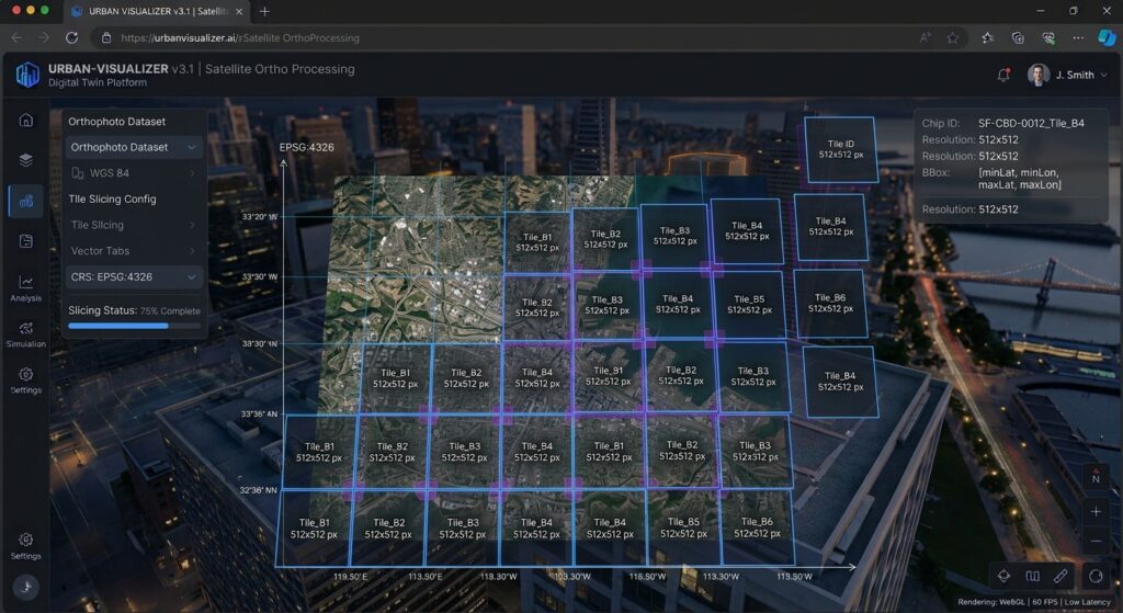
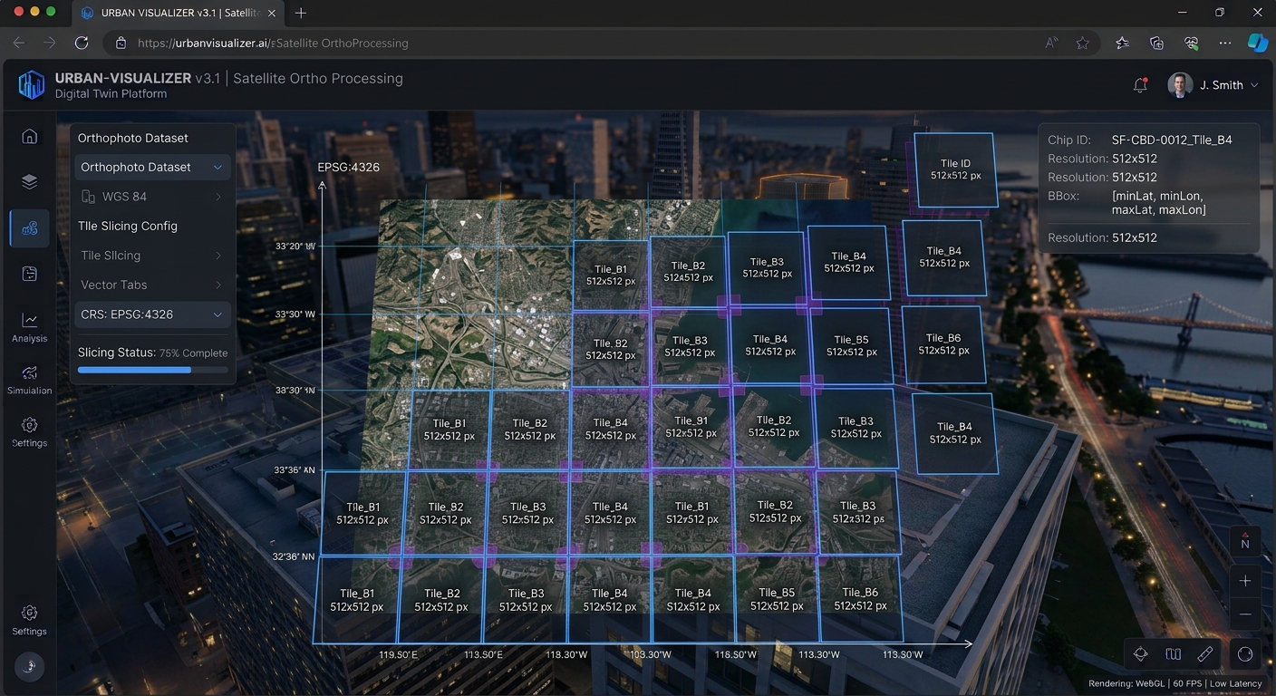
Raw GeoTIFF orthophotos carry embedded Coordinate Reference Systems (CRS) and affine transformation matrices. Breaking these files into manageable sub-chips requires preserving georeferenced metadata so that bounding box detections can later be re-projected back into real-world geographic coordinates (EPSG:4326 or local UTM zones).
1. Tiling Large GeoTIFFs with rasterio
The following production-grade Python script tiles a large GeoTIFF orthophoto into overlapping $512 \times 512$ pixel sub-chips, ensuring edge features are captured without truncation. For foundational raster manipulation techniques, refer to our comprehensive Python rasterio tutorial.
Python
import os
import rasterio
from rasterio.windows import Window
from shapely.geometry import box
import geopandas as gpd

def tile_geotiff(image_path, output_dir, tile_size=512, overlap=64):
    os.makedirs(output_dir, exist_ok=True)

    with rasterio.open(image_path) as src:
        width = src.width
        height = src.height
        transform = src.transform
        crs = src.crs

        step = tile_size - overlap

        for y in range(0, height, step):
            for x in range(0, width, step):
                # Ensure tile dimensions do not exceed raster bounds
                w = min(tile_size, width - x)
                h = min(tile_size, height - y)

                # Define spatial window
                window = Window(x, y, w, h)

                # Read raster data for window across all bands
                tile_data = src.read(window=window)

                # Compute affine transform for the specific tile
                tile_transform = rasterio.windows.transform(window, transform)

                # Update metadata for sub-chip
                meta = src.meta.copy()
                meta.update({
                    "height": h,
                    "width": w,
                    "transform": tile_transform
                })

                tile_filename = os.path.join(output_dir, f"tile_x{x}_y{y}.tif")
                with rasterio.open(tile_filename, "w", **meta) as dst:
                    dst.write(tile_data)

    print(f"Successfully tiled {image_path} into {output_dir}")

# Example invocation
# tile_geotiff("orthophoto_nairobi.tif", "./tiles", tile_size=512, overlap=64)
2. Converting Bounding Box Vectors to YOLO Label Format
YOLOv8 requires normalized bounding box text files corresponding to each image chip. Each line in a label text file represents an object annotation in the format:
$$\text{class\_id} \quad x_{\text{center}} \quad y_{\text{center}} \quad w \quad h$$
Where all coordinates and dimensions are normalized relative to the image width and height ($[0.0, 1.0]$).
Python
import numpy as np
from shapely.geometry import box
import rasterio.transform

def vector_to_yolo_labels(vector_geojson, tile_tif, output_txt):
    gdf = gpd.read_file(vector_geojson)

    with rasterio.open(tile_tif) as src:
        bounds = src.bounds
        transform = src.transform
        inv_transform = ~transform
        img_w, img_h = src.width, src.height

        tile_poly = box(bounds.left, bounds.bottom, bounds.right, bounds.top)

        # Filter vectors intersecting the tile
        intersecting = gdf[gdf.intersects(tile_poly)]

        yolo_annotations = []
        for _, row in intersecting.iterrows():
            geom = row.geometry
            # Convert polygon to bounding box
            minx, miny, maxx, maxy = geom.bounds

            # Convert spatial coordinates to pixel coordinates
            px_min, py_max = rasterio.transform.xy(transform, [miny], [minx], offset='ul')
            px_max, py_min = rasterio.transform.xy(transform, [maxy], [maxx], offset='lr')

            # Alternatively use inverse transform directly
            # Pixel space conversion
            col_min, row_max = ~transform * (minx, miny)
            col_max, row_min = ~transform * (maxx, maxy)

            x_min = max(0, min(col_min, col_max))
            x_max = min(img_w, max(col_min, col_max))
            y_min = max(0, min(row_min, row_max))
            y_max = min(img_h, max(row_min, row_max))

            if x_max <= x_min or y_max <= y_min:
                continue

            # Calculate YOLO normalized format
            x_center = ((x_min + x_max) / 2.0) / img_w
            y_center = ((y_min + y_max) / 2.0) / img_h
            w = (x_max - x_min) / img_w
            h = (y_max - y_min) / img_h

            class_id = row.get('class_id', 0)
            yolo_annotations.append(f"{class_id} {x_center:.6f} {y_center:.6f} {w:.6f} {h:.6f}")

        with open(output_txt, 'w') as f:
            f.write("\n".join(yolo_annotations))
Model Training & Inference
With our data formatted into standard PyTorch-compatible directory structures (
images/ and labels/), we can initialize and train our YOLOv8 architecture.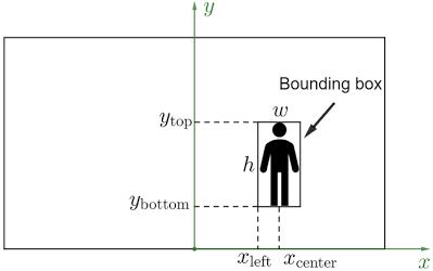
1. Setting up YOLOv8 Architecture in PyTorch
We utilize the
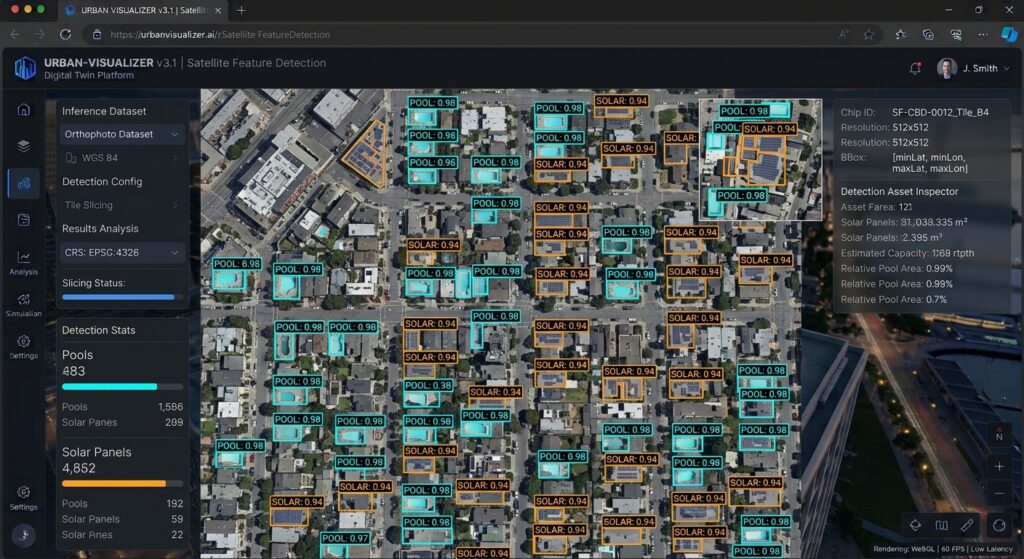
ultralytics library to configure a custom YOLOv8 model tailored for three distinct remote sensing classes: solar panels (0), swimming pools (1), and storage tanks (2). Create a configuration file named dataset.yaml:YAML
path: /path/to/dataset
train: images/train
val: images/val

names:
  0: solar_panel
  1: swimming_pool
  2: storage_tank
2. Fine-Tuning Hyperparameters for Overhead Imagery
Aerial imagery demands specific hyperparameter adjustments. Because overhead targets lack the standard horizontal bias of natural imagery, aggressive rotation, scaling, and HSV augmentations are crucial to prevent overfitting.
Python
from ultralytics import YOLO

def train_yolov8_aerial():
    # Load pretrained YOLOv8 medium model for robust feature extraction
    model = YOLO("yolov8m.pt")

    # Execute training with custom hyperparameters optimized for aerial imagery
    results = model.train(
        data="dataset.yaml",
        epochs=100,
        imgsz=512,
        batch=16,
        device=0,
        workers=8,
        optimizer="SGD",
        lr0=0.01,
        lrf=0.01,
        momentum=0.937,
        weight_decay=0.0005,
        warmup_epochs=3.0,
        box=7.5,
        cls=0.5,
        dfl=1.5,
        # Specialized augmentations for aerial perspectives
        degrees=180.0,     # Full rotation invariance for overhead objects
        translate=0.1,
        scale=0.5,         # Scale variation for varying satellite zoom levels
        shear=0.0,
        perspective=0.0,
        flipud=0.5,        # Vertical flips make sense in overhead imagery
        fliplr=0.5,
        mosaic=1.0,        # Strong mosaic augmentation for small object context
        mixup=0.1,
        copy_paste=0.1
    )

    print("Training complete. Best weights saved to runs/detect/train/weights/best.pt")

if __name__ == "__main__":
    # train_yolov8_aerial()
    pass
3. Running Inference and Stitching Tile Predictions into GeoJSON Vectors
Once trained, running inference across massive spatial scenes requires iterating over all tiles, performing non-max suppression (NMS), and transforming pixel bounding boxes back into geographic coordinates. We then export these detections into unified GeoJSON vectors.
Python
import glob
import json
from shapely.geometry import box as shapely_box, mapping
import geopandas as gpd

def predict_and_stitch(weights_path, tile_dir, output_geojson):
    model = YOLO(weights_path)
    features = []

    tile_paths = glob.glob(os.path.join(tile_dir, "*.tif"))

    for tile_path in tile_paths:
        with rasterio.open(tile_path) as src:
            transform = src.transform
            crs = src.crs

            # Run inference on individual tile
            results = model.predict(tile_path, conf=0.45, iou=0.5, verbose=False)
            boxes = results[0].boxes

            for box_tensor in boxes:
                xyxy = box_tensor.xyxy[0].cpu().numpy() # [x1, y1, x2, y2] in pixels
                conf = float(box_tensor.conf[0].cpu().numpy())
                cls_id = int(box_tensor.cls[0].cpu().numpy())

                x1, y1, x2, y2 = xyxy

                # Transform pixel coordinates to geospatial coordinates
                ul_x, ul_y = transform * (x1, y1)
                lr_x, lr_y = transform * (x2, y2)

                # Create shapely polygon for bounding box
                geom = shapely_box(min(ul_x, lr_x), min(ul_y, lr_y), max(ul_x, lr_x), max(ul_y, lr_y))

                features.append({
                    "geometry": mapping(geom),
                    "properties": {
                        "class_id": cls_id,
                        "class_name": model.names[cls_id],
                        "confidence": conf,
                        "source_tile": os.path.basename(tile_path)
                    }
                })

    # Create GeoDataFrame and save to GeoJSON
    gdf = gpd.GeoDataFrame.from_features(features, crs=crs)
    gdf.to_file(output_geojson, driver="GeoJSON")
    print(f"Inference complete. Saved {len(gdf)} detections to {output_geojson}")
Advanced Geospatial Extensions & Ecosystem Integration
For advanced remote sensing operations, object detection outputs often feed into broader spatial workflows:
-
Semantic Segmentation Refinement: Pair YOLOv8 bounding box coordinates with SAM 2 building footprint extraction models to derive precise vector polygons rather than bounding boxes.
-
Urban Dynamics & Flow: Aggregate detected vehicular assets over time using Graph Neural Networks for traffic prediction models to model metropolitan congestion.
Conclusion
Implementing a robust YOLOv8 geospatial object detection pipeline in PyTorch bridges the gap between state-of-the-art computer vision and enterprise GIS analysis. By properly handling large orthophoto tiling via
rasterio, configuring rotation-invariant augmentations, and re-projecting bounding box predictions back into georeferenced vector formats, remote sensing teams can automate large-scale asset inventory with exceptional speed and precision.Want to master advanced computer vision workflows? Bookmark this guide on YOLOv8 geospatial object detection, or reach out to our team if you need expert help with your advanced GIS assignments.