

Spatial Point Pattern Analysis of Crime Data Using Kernel Density Estimation (KDE) in Python

Understanding the spatial distribution of point events is a foundational pillar of quantitative geography, urban criminology, and emergency resource allocation. Whether analyzing urban crime incidents, vehicular collisions, or disease outbreaks, spatial analysts seek to uncover underlying clustering patterns rather than merely observing discrete points on a map.
Traditional approaches—such as aggregating point events into arbitrary grid cells or administrative polygons and computing simple counts—suffer from severe limitations, including the Modifiable Areal Unit Problem (MAUP) and abrupt boundary artifacts. Kernel Density Estimation (KDE) solves these challenges by transforming discrete spatial points into a continuous probability density surface.
In this comprehensive tutorial, we will construct an end-to-end Python pipeline to compute 2D Gaussian Kernel Density Estimation on urban crime incident coordinates, optimize bandwidth parameters, visualize contours over a street network, and rasterize output surfaces into cloud-optimized GeoTIFF files.
Prerequisites & Python Setup
To implement our spatial point pattern analysis pipeline, we rely on a robust geospatial and scientific Python stack. Ensure your virtual environment contains the following core packages:
-
geopandas: For handling vector spatial data and coordinate reference systems (CRS). -
shapely: For geometric manipulations and bounding box calculations. -
numpy: For numerical grid generation and matrix operations. -
scipy: Specificallyscipy.stats.gaussian_kdefor executing the 2D kernel density estimation. -
matplotlib: For visualization and plotting contour overlays. -
rasterio: For exporting continuous raster arrays into georeferenced GeoTIFF formats.
You can install the required dependencies via pip:
Bash
pip install geopandas shapely numpy scipy matplotlib rasterio
Step 1: Loading Spatial Point Data and Re-Projecting to a Metric CRS
Spatial distance calculations—and by extension, kernel bandwidth sizing—require units of measurement that reflect true physical distances on the Earth’s surface (e.g., meters or feet). Raw GPS coordinates stored in geographic coordinate systems (such as WGS 84, EPSG:4326) measure locations in degrees of latitude and longitude, distorting spatial distance across varying latitudes.
Our first step is to load a GeoJSON or Shapefile containing point crime records and re-project the dataset into a local metric coordinate reference system, such as UTM (Universal Transverse Mercator).
Python
import geopandas as gpd
from shapely.geometry import Point

# Load crime incident points from a sample GeoJSON file
# For demonstration, assume our dataset contains point geometries representing incidents
input_path = "urban_crime_incidents.geojson"
gdf = gpd.read_file(input_path)

print(f"Original CRS: {gdf.crs}")
print(f"Total crime records loaded: {len(gdf)}")

# Re-project from WGS84 (EPSG:4326) to a local Metric CRS (e.g., UTM Zone 37S - EPSG:32737)
# Note: Choose the appropriate UTM zone or local projected CRS for your study area
projected_crs = "EPSG:32737"
gdf_projected = gdf.to_crs(projected_crs)

print(f"Re-projected to metric CRS: {gdf_projected.crs}")
Step 2: Setting Optimal Bandwidth Parameters
The bandwidth parameter ($h$), also known as the smoothing parameter or search radius, is the single most influential setting in KDE. It dictates the spatial extent over which an individual point’s influence is distributed across the surrounding surface.
-
Undersmoothing (Too small $h$): Produces a spiky surface that mirrors individual points, failing to reveal broader structural hotspots and overemphasizing random noise.
-
Oversmoothing (Too large $h$): Overly smooths the surface, masking localized high-density clusters and blending distinct hot spots into a homogenous blur.
Silverman’s Rule of Thumb
A standard heuristic for bandwidth selection in two dimensions is Silverman’s rule of thumb, which calculates bandwidth based on the standard deviation of coordinates and sample size ($n$):
$$h = \left( \frac{4}{d + 2} \right)^{\frac{1}{d + 4}} \cdot n^{-\frac{1}{d + 4}} \cdot \sigma$$
Where $d = 2$ (two-dimensional spatial coordinates) and $\sigma$ is the mean standard deviation of the $X$ and $Y$ coordinates.
Python
import numpy as np

def calculate_silverman_bandwidth(coordinates):
    """
    Calculates 2D bandwidth using Silverman's Rule of Thumb.
    coordinates: numpy array of shape (N, 2) representing [X, Y] in meters.
    """
    n = coordinates.shape[0]
    d = 2  .0 # Two spatial dimensions

    # Calculate standard deviation of X and Y coordinates
    sigma_x = np.std(coordinates[:, 0])
    sigma_y = np.std(coordinates[:, 1])
    mean_sigma = (sigma_x + sigma_y) / 2.0

    # Silverman's formula for d=2
    h = ( (2.0 / (d + 2.0)) ** (1.0 / (d + 4.0)) ) * (n ** (-1.0 / (d + 4.0))) * mean_sigma
    return h

# Extract metric X, Y arrays from projected GeoDataFrame
coords = np.array([[geom.x, geom.y] for geom in gdf_projected.geometry])
bandwidth_meters = calculate_silverman_bandwidth(coords)

print(f"Calculated Silverman Optimal Bandwidth: {bandwidth_meters:.2f} meters")
Step 3: Running 2D Gaussian KDE Using scipy.stats.gaussian_kde
With our coordinates prepared in metric units and the optimal bandwidth established, we can compute the Kernel Density Estimation using
scipy.stats.gaussian_kde. We instantiate the KDE object, pass our transposed coordinate array, and evaluate the density across a regular grid spanning the bounding box of our study area.Python
from scipy.stats import gaussian_kde

# Transpose coordinates to shape (2, N) as required by scipy gaussian_kde
kde_input = coords.T

# Initialize Gaussian KDE with custom bandwidth scaling
# Scipy allows setting covariance factor directly or scaling standard scott/silverman methods
# Here we scale covariance factor based on our calculated bandwidth ratio
eval_cov = (bandwidth_meters / np.std(coords)) ** 2
kde = gaussian_kde(kde_input, bw_method=eval_cov)

# Define grid resolution (e.g., 20-meter pixel grid)
cell_size = 20.0  # meters

xmin, ymin, xmax, ymax = gdf_projected.total_bounds
# Buffer bounds slightly to prevent edge artifacts during raster generation
buffer = bandwidth_meters * 2
xmin -= buffer
xmax += buffer
ymin -= buffer
ymax += buffer

x_grid = np.arange(xmin, xmax, cell_size)
y_grid = np.arange(ymin, ymax, cell_size)
xx, yy = np.meshgrid(x_grid, y_grid)

# Flatten grid points for evaluation
grid_coords = np.vstack([xx.ravel(), yy.ravel()])

print(f"Evaluating KDE across prediction grid of shape {xx.shape} ({grid_coords.shape[1]} total cells)...")

# Evaluate density estimator on grid points
z_density = kde(grid_coords).reshape(xx.shape)

print("KDE evaluation completed successfully.")
Step 4: Visualizing Hotspots and Rasterizing Outputs to GeoTIFF
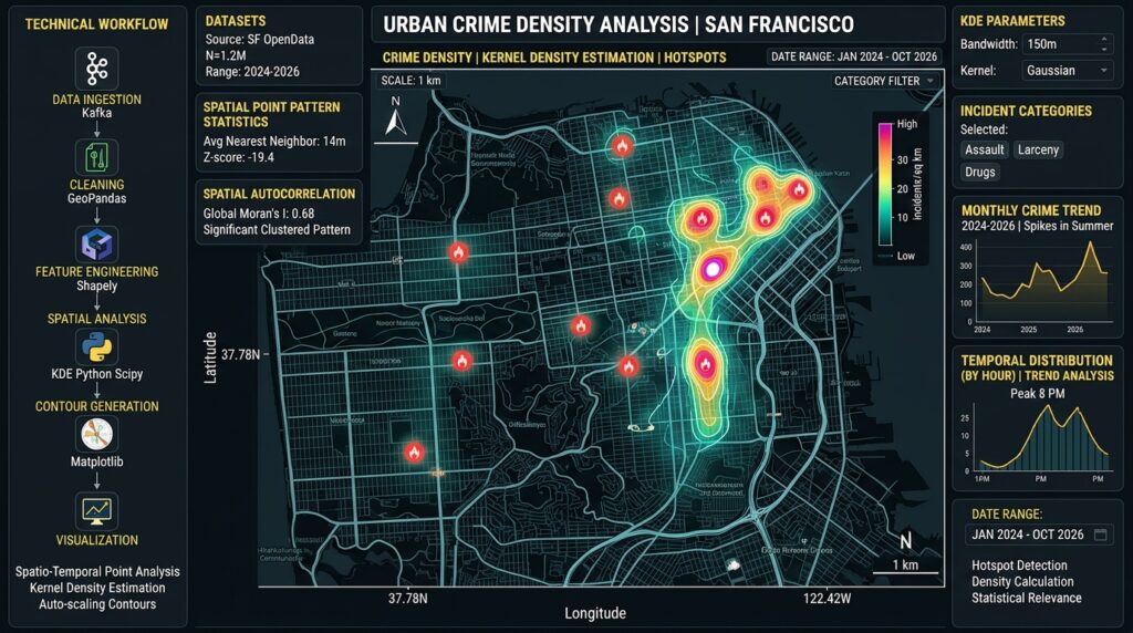
Once we have evaluated our density surface, we can visualize the resulting hotspots using
matplotlib with custom colormaps and contour overlays. Furthermore, professional GIS workflows require exporting these analytical surfaces as georeferenced raster files (.tif) for integration with desktop software such as QGIS or ArcGIS Pro, or for serving via web-mapping servers like GeoServer.Python
import matplotlib.pyplot as plt
import rasterio
from rasterio.transform import from_origin

# 1. Plotting the KDE Heatmap with Matplotlib
fig, ax = plt.subplots(figsize=(10, 10))

# Plot continuous density surface
contour = ax.contourf(xx, yy, z_density, levels=25, cmap='inferno')
cbar = fig.colorbar(contour, ax=ax, shrink=0.7)
cbar.set_label('Crime Incident Density (Points / $m^2$)', fontsize=12)

# Overlay original crime incident points
ax.scatter(coords[:, 0], coords[:, 1], c='cyan', s=5, alpha=0.5, label='Crime Incidents')

ax.set_title('Spatial Point Pattern Analysis: Crime Incident KDE Hotspots', fontsize=14, fontweight='bold')
ax.set_xlabel(f'Easting ({projected_crs})', fontsize=11)
ax.set_ylabel(f'Northing ({projected_crs})', fontsize=11)
ax.legend(loc='upper right')
ax.set_aspect('equal')

plt.tight_layout()
plt.savefig('crime_kde_hotspots.png', dpi=300)
plt.show()


# 2. Rasterizing and Exporting to GeoTIFF using Rasterio
# Note: Rasterio requires top-left origin coordinates (ymax for North-up raster)
transform = from_origin(xmin, ymax, cell_size, cell_size)

# Ensure density values are stored in float32 format
raster_data = z_density.astype(np.float32)

output_tiff = "crime_density_surface.tif"

with rasterio.open(
    output_tiff,
    'w',
    driver='GTiff',
    height=raster_data.shape[0],
    width=raster_data.shape[1],
    count=1,
    dtype=raster_data.dtype,
    crs=projected_crs,
    transform=transform,
) as dst:
    dst.write(raster_data, 1)

print(f"Successfully exported KDE density surface to {output_tiff}")
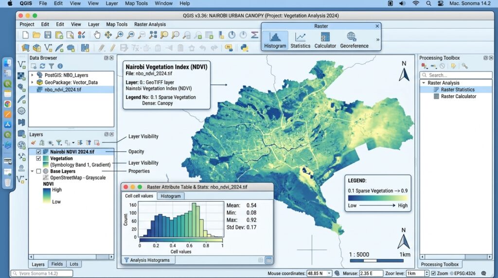
Advanced Analytical Considerations in Point Pattern Analysis
While Kernel Density Estimation provides an intuitive continuous surface of event intensity, quantitative spatial analysts must consider supplementary statistical tests to validate observed clustering patterns:
-
Spatial Randomness Testing via Monte Carlo Simulations: Before concluding that an area is a statistically significant hotspot, analysts often test against Complete Spatial Randomness (CSR) using spatial point pattern simulations (Monte Carlo) to evaluate whether observed clusters deviate significantly from a Poisson point process.
-
Nearest Neighbor Distance Metrics: To measure whether point distributions exhibit clustering, dispersion, or randomness prior to density mapping, computing the Nearest Neighbor Index (NNI) provides a robust global metric comparing mean observed nearest-neighbor distances against expected theoretical random distributions.
-
Boundary Effects: KDE surfaces can suffer from boundary bias near study area edges because search windows are truncated outside the boundary. Applying adaptive bandwidths or boundary correction weighting vectors helps mitigate edge underestimation.
Conclusion
Spatial point pattern analysis using Kernel Density Estimation bridges raw coordinate geometry and actionable geographic intelligence. By moving beyond naive grid aggregation and implementing custom metric projections, optimal bandwidth selection via Silverman’s rule, and efficient array evaluation with
scipy, spatial analysts can isolate true crime hotspots. Exporting these outputs as standardized GeoTIFF layers bridges advanced Python data science workflows with operational GIS infrastructure, empowering law enforcement agencies and urban planners to deploy resources efficiently.