Table of Contents

Calculating NDVI and Vegetation Health in ArcGIS Pro: A Complete Walkthrough

Introduction: What Is NDVI?

The Normalized Difference Vegetation Index (NDVI) is a remote sensing indicator used to assess vegetation greenness and relative vigor using multispectral satellite imagery. It is widely applied in agricultural monitoring, forestry, environmental management, drought assessment, and land-cover analysis.

NDVI works by measuring the difference between how vegetation reflects near-infrared radiation and how it absorbs red light. Healthy green leaves typically absorb much of the red light for photosynthesis while reflecting a relatively large proportion of near-infrared radiation. This contrast helps distinguish vegetation from many non-vegetated surfaces.

The NDVI formula

The standard mathematical equation is:

[
\mathrm{NDVI}=\frac{NIR-Red}{NIR+Red}
]

Where:

NIR: Reflectance measured in the near-infrared spectral band.
Red: Reflectance measured in the red spectral band.

NDVI values theoretically range from -1 to +1. In general, higher positive values indicate greener vegetation, whereas values near zero often correspond to bare soil, built-up surfaces, or sparse vegetation. Negative values may indicate water, clouds, snow, or other surfaces with little vegetation. Interpretation depends on the sensor, season, land cover, and image quality.

NDVI is therefore a useful indicator of vegetation greenness, but it is not a direct measurement of plant health, disease, or agricultural yield. These outcomes require additional contextual information and, in many cases, field observations.

1. Data Requirements

Before calculating NDVI in ArcGIS Pro, obtain suitable multispectral satellite imagery containing both red and near-infrared bands.

Two commonly used sources are Landsat 8/9 and Sentinel-2.

1.1 Landsat 8 and Landsat 9

Landsat 8 and 9 provide multispectral imagery suitable for regional vegetation monitoring. Their operational land imager reflective bands generally have a spatial resolution of 30 meters. The relevant bands are:

Band	Spectral region	Use in NDVI
Band 4	Red	Red reflectance
Band 5	Near-infrared (NIR)	NIR reflectance

For standard Landsat 8/9 NDVI, use Band 5 as NIR and Band 4 as red. Confirm the sensor and product specifications before processing. USGS band specifications.

For quantitative analysis, surface reflectance products are generally preferable to uncorrected digital numbers because they account for atmospheric effects and provide more meaningful reflectance measurements.

Important: Landsat Collection 2 Level-2 surface reflectance data stored as integer values require the documented scale factor and additive offset when converting the stored values to reflectance. The USGS specifies:

[
SR=(DN \times 0.0000275)-0.2
]

Apply the appropriate scaling and mask fill pixels before calculating NDVI. USGS scaling guidance.

1.2 Sentinel-2

Sentinel-2 provides multispectral imagery with several spatial resolutions. Its commonly used NDVI bands are:

Band	Spectral region	Spatial resolution
B04	Red	10 m
B08	Near-infrared (NIR)	10 m

These bands support vegetation mapping at a finer spatial resolution than the standard Landsat reflective bands. See the Copernicus Sentinel-2 band specifications.

1.3 Prepare your project files

For this walkthrough, assume the following inputs:

GIS_Project/
│
├── Landsat_or_Sentinel_Image
├── Study_Area.gpkg
├── Agricultural_Parcels.gpkg
└── NDVI_Results/

The example uses a multiband raster for the built-in NDVI method and individual red and NIR rasters for the manual Raster Calculator method.

Before proceeding, make sure your imagery covers the study area, has appropriate reflectance values, and has been checked for clouds and cloud shadows.

2. Step One: Load Satellite Imagery into ArcGIS Pro

The first step is to add the satellite imagery to your map and confirm which bands are available.

Step 1.1: Open your project

Launch ArcGIS Pro and open an existing project or create a new map project.

From the ribbon, select:

Map → Add Data

Browse to the directory containing your satellite imagery and add the relevant raster dataset or raster product.

For example, you might add a Landsat multispectral raster, a Sentinel-2 raster product, or individual band files.

Step 1.2: Inspect the raster properties

In the Contents pane, right-click the image layer and select:

Properties → Source

Check the following:

Coordinate system.
Raster dimensions and pixel size.
Number of bands.
Pixel data type.
Extent and spatial coverage.

If you are working with individual band files, confirm their identities from their filenames and metadata. Do not assume that the fourth layer in a raster stack is necessarily the fourth band of the original satellite sensor.

Step 1.3: Display a false-color composite

For visual inspection, you can use a false-color composite in which NIR is displayed in the red channel, red in the green channel, and green in the blue channel.

For Landsat 8/9, a conventional false-color composite uses:

Red display channel: Band 5 (NIR).
Green display channel: Band 4 (red).
Blue display channel: Band 3 (green).

This combination often makes healthy vegetation appear bright red, helping you distinguish vegetated areas from many non-vegetated surfaces.

For Sentinel-2, the corresponding combination is generally B08, B04, and B03.

A false-color composite is useful for visual inspection, but it is not the NDVI calculation itself.

3. Step Two: Calculating NDVI and Vegetation Health in ArcGIS Pro

ArcGIS Pro provides an NDVI raster function that calculates the index from red and near-infrared bands.

In current ArcGIS Pro versions, the function is available through the Imagery tab and the Indices gallery, or through the Raster Functions pane. The exact ribbon arrangement can differ by version and interface configuration. See the official ArcGIS Pro NDVI function documentation.

Step 3.1: Select the multiband raster

In the Contents pane, select the multispectral raster containing the red and NIR bands.

The raster needs to expose the appropriate spectral bands, either as a supported multiband raster or an imagery product.

If your red and NIR bands are separate single-band files, you can use the manual Raster Calculator method in Section 4 or create a suitable multiband raster first.

Step 3.2: Open the NDVI function

Use the ribbon path:

Imagery → Indices → NDVI

If the NDVI option is not visible, open:

Imagery → Raster Functions

Search for NDVI in the Raster Functions pane and open the NDVI function.

Step 3.3: Set the band parameters

In the NDVI function parameters, identify the bands representing red and near-infrared radiation.

For Landsat 8/9, use:

Parameter	Sensor band
Visible Band ID	Band 4 — red
Infrared Band ID	Band 5 — NIR

For Sentinel-2, use:

Parameter	Sensor band
Visible Band ID	B04 — red
Infrared Band ID	B08 — NIR

The function’s band IDs refer to positions or identities within the input raster, depending on how the raster is organized. Verify the actual input band mapping rather than blindly entering sensor band numbers. A composite containing only selected bands may number them differently from the original satellite product.

Step 3.4: Select the scientific output option

Where the interface offers a Scientific Output setting, enable it to retain conventional NDVI values between -1 and +1.

Without scientific output, the NDVI raster function can return a transformed range:

[
NDVI_{\mathrm{display}}=
\left(\frac{NIR-Red}{NIR+Red}\right)\times100+100
]

This produces values between approximately 0 and 200 rather than -1 and +1.

Both representations can be displayed, but you must know which one you have before interpreting statistics or applying classification thresholds. ArcGIS Pro NDVI function reference.

Step 3.5: Inspect the resulting NDVI layer

Run or apply the function according to the controls presented in your ArcGIS Pro version.

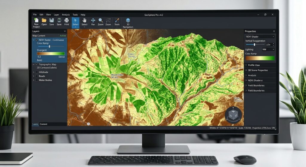
The output should emphasize differences in vegetation greenness across the scene. Inspect the image for:

High NDVI values in areas of vigorous green vegetation.
Lower positive values over sparse vegetation.
Values close to zero over many bare or built-up surfaces.
Negative values in some water, cloud, or snow pixels.

Raster functions may initially create a function raster layer that is evaluated during display rather than a permanent raster file. For a durable analytical output, use the available export or save operation to write the NDVI result to disk.

A useful filename might be:

NDVI_BuiltIn.tif

4. Step Three: Calculate NDVI Manually with Raster Calculator

The manual method gives you more control over the equation, input data preparation, and handling of invalid pixels.

ArcGIS Pro’s Raster Calculator uses map algebra expressions. It is available through the Geoprocessing pane and requires a Spatial Analyst or Image Analyst license. See the Raster Calculator documentation.

Step 4.1: Prepare the red and NIR bands

Add the appropriate red and NIR raster layers to your map.

For Landsat 8/9, the inputs are:

Red = Band 4
NIR = Band 5

For Sentinel-2, the inputs are:

Red = B04
NIR = B08

Ensure the rasters represent compatible reflectance values and have the same spatial alignment, coverage, and suitable pixel sizes.

If you are using Landsat Collection 2 Level-2 surface reflectance files containing stored integer values, prepare scaled reflectance rasters before calculating NDVI.

Open Raster Calculator and convert the red band:

Float("SR_B4") * 0.0000275 - 0.2

Save the result as Red_Reflectance.

For the NIR band:

Float("SR_B5") * 0.0000275 - 0.2

Save the result as NIR_Reflectance.

Here, SR_B4 and SR_B5 are example layer names. Replace them with the actual names of your input rasters. Mask fill pixels before applying these expressions, because fill values must not be interpreted as real surface reflectance.

For other satellite products, consult the provider’s documentation to determine whether scaling is needed.

Step 4.2: Open Raster Calculator

In ArcGIS Pro, go to:

Analysis → Tools

Search for:

Raster Calculator

Open the tool from the Geoprocessing results.

You should see an expression area in which you can enter the NDVI formula.

Step 4.3: Enter the NDVI expression

If your input rasters already contain valid red and NIR reflectance values, enter:

SetNull(
    ("NIR_Reflectance" + "Red_Reflectance") == 0,
    Float("NIR_Reflectance" - "Red_Reflectance") /
    Float("NIR_Reflectance" + "Red_Reflectance")
)

Replace the example layer names with the names in your Contents pane. Selecting or double-clicking the raster names in the tool’s raster list can help avoid typing errors.

This expression performs three operations:

Adds NIR and red reflectance to create the denominator.
Subtracts red reflectance from NIR reflectance to create the numerator.
Divides the numerator by the denominator to calculate NDVI.

The Float() function helps ensure floating-point division rather than unintended integer division. SetNull() sets pixels with a zero denominator to NoData instead of attempting an undefined division.

Note: This expression handles a zero denominator; it does not replace cloud masking or removal of invalid source pixels. Perform those quality-control steps separately.

Step 4.4: Set the output raster

In the Output raster parameter, choose a geodatabase location or a suitable raster file path.

For example:

NDVI_Manual.tif

Where relevant, set processing environments so the cell size, output extent, and snap raster align with your analysis. This is particularly important if you will compare multiple rasters or calculate zonal statistics.

Click Run.

Step 4.5: Verify the output

Inspect the resulting raster and its properties.

For a standard scientific NDVI raster, the values should ordinarily fall within -1 to +1, allowing for minor floating-point precision effects.

If the output looks entirely positive, entirely negative, or otherwise implausible, check the input band selection, scaling, NoData treatment, and expression.

5. Step Four: Apply a Color Ramp to Highlight Vegetation

A suitable color scheme makes it easier to interpret spatial patterns in the NDVI raster.

Step 5.1: Open the Symbology pane

In the Contents pane, right-click your NDVI raster and choose:

Symbology

For a continuous NDVI surface, use Stretch symbology where available. A divergent or vegetation-oriented color scheme can distinguish low values from high values.

For example, a practical display may use:

Red or brown for very low NDVI values.
Yellow or pale green for intermediate values.
Dark green for higher NDVI values.

Ensure the legend labels reflect the actual output range. If the built-in function produced a 0–200 representation, do not label those values as though they were the original -1 to +1 NDVI values.

Step 5.2: Adjust the display range

If scientific NDVI values are used, a display range from -1 to +1 can provide a consistent starting point. However, many scenes contain few pixels near the theoretical extremes.

You may adjust the stretch to make local differences easier to see, but document any nonstandard range if the map is used for research or comparison.

Avoid changing the display stretch between dates when the purpose is direct visual comparison, unless the adjustment is explicitly justified and clearly documented.

Step 5.3: Optionally classify NDVI into categories

You can use classified symbology or a reclassification workflow to summarize vegetation into classes.

The following ranges are illustrative starting points, not universal definitions of vegetation health:

NDVI range	Possible interpretation
Below 0	Often water, clouds, snow, or other non-vegetated surfaces
0.00–0.20	Bare ground or very sparse vegetation
0.20–0.40	Sparse to moderately green vegetation
0.40–0.60	Moderate to relatively dense vegetation
0.60–1.00	Often dense, vigorous green vegetation

These ranges vary with crop type, canopy structure, soil background, season, moisture, and the satellite sensor. Choose thresholds suited to the study context and justify them before using the classes to make agricultural or ecological conclusions.

For agricultural monitoring, a field with an NDVI of 0.45 is not automatically unhealthy. Its meaning depends on what is being grown, the growth stage, local conditions, and reference observations.

6. Step Five: Calculate Zonal Statistics for Agricultural Parcels

A vegetation map shows where NDVI values are high or low. Zonal statistics summarize those pixel values within defined areas, such as farms, agricultural parcels, watersheds, or administrative zones.

ArcGIS Pro provides the Zonal Statistics as Table tool for this purpose. It requires a Spatial Analyst or Image Analyst license. Official tool reference.

Step 6.1: Load the zone polygons

Add your agricultural parcel or administrative boundary dataset to the map.

For example:

Agricultural_Parcels

Ensure that each polygon has an identifier field that uniquely identifies the relevant zone, such as Parcel_ID.

Step 6.2: Open Zonal Statistics as Table

Go to:

Analysis → Tools

Search for:

Zonal Statistics as Table

Open the tool from the search results.

Step 6.3: Configure the parameters

Set the parameters as follows:

Parameter	Example value
Input Raster or Feature Zone Data	`Agricultural_Parcels`
Zone Field	`Parcel_ID`
Input Value Raster	`NDVI_Manual`
Output Table	`NDVI_Parcel_Stats`
Ignore NoData in Calculations	`DATA`
Statistics Type	`MEAN` or `ALL`, as appropriate

Replace the examples with your actual layer and field names.

Using DATA instructs the tool to ignore NoData cells when calculating statistics. This does not remove clouds that were incorrectly retained as valid pixel values, so proper cloud and shadow masking remains essential.

If you select ALL, the tool calculates the supported suite of statistics rather than just the mean.

Step 6.4: Set raster-processing environments

When polygon boundaries are converted internally to raster zones, cell size and pixel alignment matter.

For more consistent results:

Use the NDVI raster as the snap raster where appropriate.
Set a suitable cell size based on the NDVI raster.
Check the output coordinate system and processing extent.
Make sure the polygons overlap the raster and that the chosen zone field identifies the intended zones.

This helps ensure that your zonal summaries use consistent raster cells.

Step 6.5: Run the tool

Click Run.

The output table will contain a record for each zone and the statistics calculated for its NDVI pixels.

For example, you may receive results similar to:

Parcel_ID	MEAN	MIN	MAX
P001	0.68	0.32	0.84
P002	0.42	0.11	0.66
P003	0.27	0.02	0.49

These values are hypothetical and illustrate the structure of the output. They are not measurements from an actual satellite scene.

The mean NDVI provides a simple summary of the average greenness of the pixels assigned to each parcel. Minimum and maximum values help identify variation within a zone, although they can also be affected by outliers and residual image contamination.

Step 6.6: Join the results back to the polygons

To map the results by parcel, join the statistics table to the original parcel layer using the common identifier field.

You can use:

Analysis → Tools → Join Field

Set the input table or layer to Agricultural_Parcels, the input join field to Parcel_ID, the join table to NDVI_Parcel_Stats, and the join field in that table to the corresponding parcel identifier.

Run the tool and confirm that the output polygons contain the expected summary fields.

You can now symbolize the polygons by mean NDVI, create a parcel-level statistics table, or export the results for further analysis.

7. Common Errors and Troubleshooting

Error 1: Incorrect band indices

Problem: The NDVI map appears inverted or does not resemble the expected vegetation pattern.

Likely cause: The red band and near-infrared band were swapped, or the software was given the wrong band IDs.

Solution: Verify the band identities in the source metadata. For Landsat 8/9, standard NDVI uses Band 5 for NIR and Band 4 for red. For Sentinel-2, use B08 for NIR and B04 for red. Confirm how those bands are organized within the actual input raster.

Error 2: Cloud contamination

Problem: Cloud-covered regions produce unusual or misleading NDVI values.

Likely cause: Clouds, cloud shadows, and other poor-quality pixels were included in the analysis.

Solution: Use appropriate quality information to mask clouds and shadows. Landsat products provide quality-assessment bands, while Sentinel-2 products provide classification information that can be used for masking. Exclude invalid pixels before calculating zonal statistics. The Copernicus Sentinel-2 documentation describes the use of scene classification information to exclude cloud-affected observations.

Error 3: Implausible NDVI values from Landsat Collection 2 data

Problem: Calculated values look unreasonable even though the correct spectral bands were selected.

Likely cause: Integer surface reflectance values were used without accounting for the scale factor and additive offset.

Solution: Confirm the product level and apply the documented scale factor and offset where required. Do not automatically assume all satellite products use the same scaling convention. Refer to the USGS Landsat scaling instructions.

Error 4: Raster Calculator fails

Problem: The expression fails or produces an invalid output.

Likely cause: A raster layer name is misspelled, parentheses are missing, the expression has a syntax error, or the required extension is unavailable.

Solution: Insert raster names using the Raster Calculator interface, check that parentheses are balanced, verify that floating-point expressions are used, and confirm that the necessary license is available.

Error 5: The NDVI layer has values between 0 and 200

Problem: The raster does not appear to contain negative values.

Likely cause: The default NDVI function output has been transformed for display or storage.

Solution: Check the function parameters and activate Scientific Output where available. Otherwise, convert the transformed values back to standard NDVI values using:

[
NDVI=\frac{V}{100}-1
]

where (V) is a value from the transformed 0–200 representation. Confirm that the layer is in this representation before applying the conversion.

Error 6: Zonal statistics contain unexpected NoData results

Problem: Some agricultural parcels have missing or incomplete summaries.

Likely cause: The parcels fall outside the raster extent, contain no valid pixels, or overlap areas masked as NoData.

Solution: Check the spatial alignment, extent, zone identifiers, and quality mask. Ensure that each zone contains valid NDVI cells before interpreting the summary statistics.

8. Summary

Calculating NDVI and vegetation health indicators in ArcGIS Pro involves preparing multispectral imagery, selecting the correct spectral bands, calculating the index, choosing an appropriate symbology, and summarizing values across meaningful geographic zones.

The standard equation is:

[
\mathrm{NDVI}=\frac{NIR-Red}{NIR+Red}
]

The essential workflow is:

Add and inspect Landsat 8/9 or Sentinel-2 imagery.
Verify band identities, reflectance scaling, and image quality.
Use Imagery → Indices → NDVI, or access the NDVI raster function through the Raster Functions pane.
Alternatively, use Analysis → Tools → Raster Calculator to calculate NDVI explicitly.
Apply a color ramp with a clearly defined value range.
Run Zonal Statistics as Table to summarize NDVI within agricultural parcels or administrative areas.
Validate the output and document the parameters used.

The most important considerations are correct band selection, cloud and shadow masking, reflectance scaling, and consistent interpretation of NDVI values.

NDVI is a valuable indicator of vegetation greenness and relative vigor, but it should not be treated as a complete diagnosis of vegetation health on its own. Combining the index with seasonal information, field observations, land-cover context, and other relevant indicators provides a stronger foundation for agricultural and environmental analysis.